Biostatistics for MS2 Students

Part 3: Statistical Hypothesis Testing

Statistical hypothesis testing describes a methodology by which researchers infer conclusions about a general population, using data from a limited sample and calculations involving probability. The motivation is to find a way to do this which is objective and unbiased.

Example

Cooper et al published a study in 1993 which consisted of a trial of the drug Zidovudine (AZT) as a treatment to prevent HIV from progressing to disease (ie. the patient becoming symptomatic). In the study, 936 patients with asymptomatic HIV infection were treated with either AZT or with a placebo for a period of three years. The endpoint was progression of disease.

Of the 936 patients, 475 were treated with AZT and 461 with the placebo. The primary results can be summarized in the following table:

		Disease status
		Symptomatic	Not symptomatic	Total
Treatment	AZT	76	399	475
Treatment	Placebo	129	332	461
	Total	205	731	936

Hypothesis testing is always formulated as testing one hypothesis against another. In this example, the hypothesis the investigators want to support is that AZT benefits patients who are HIV+ by making it less likely that they will progress to disease. In the language of hypothesis testing, we formulate a null hypothesis, denoted \(H_0\) which is the hypothesis we would conservatively believe if we had no evidence to the contrary. Against this, we formulate the alternative hypothesis, \(H_a\), which is the hypothesis we want to demonstrate. In our example, we have:

\(H_0\) : AZT makes no difference to the chances of HIV progressing to disease
\(H_a\) : AZT affects the chances of HIV progressing to disease

The first point to make here is that no matter how well-designed your experiment, and no matter how much data you collect:

You can never definitively prove your hypothesis with your data.

The reason for this is that our hypothesis concerns the population (in this case, all HIV-infected patients, present and future), while our data are taken from a sample.

From the table above, we can calculate the percentage of patients who receive AZT who progress to symptomatic disease as 76/475=16%. By contrast, the percentage of patients who receive the placebo who progress to symptomatic disease is 129/461=28%.

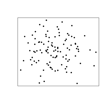
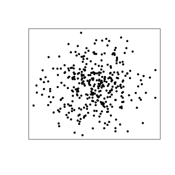
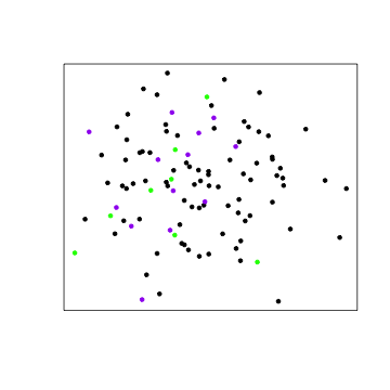
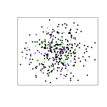
To demonstrate these results are possible if the null hypothesis is true, lets suppose that the proportion of patients in the entire population who progress to disease is 22%, no matter what treatment the receive. The picture would look something like this:

Symptomatic	Not Symptomatic

We then randomly select 475 patients who will receive AZT, and 461 who will receive the placebo. Our patients, of course, come from a single group (we don't know who progresses to disease and who doesn't until the end of the trial), so these random selections are just made from the group as a whole. Since the sampling is random, any configuration is possible. Denoting AZT patients in green and placebo in purple (with one dot representing 10 patients), simply by random sampling we might end up with

Symptomatic	Not Symptomatic

This would give us the results in the table, despite the fact that the null hypothesis is true, i.e. that, in this scenario, there is no effect on the chances of progression to disease of AZT.

Of course, intuitively, it seems that the scenario of being this "unlucky" in our choice of sample is extremely unlikely. What we'd ideally like to do is examine our data and calculate the probability the null hypothesis is false. Unfortunately:

There is no objective, unbiased way to calculate the probability the null hypothesis is true (or false) from the data from a sample

In 1925, the statistician and geneticist Ronald Fisher proposed the following approach:

Calculate the probability of observing data at least as extreme as the data that was actually observed, under the assumption that the null hypothesis is true. If this probability is small, i.e. if it would be unlikely to observe the data you actually observed, then this provides strong evidence to reject the null hypothesis and conclude tha the alternative hypothesis is true.

In our example, this means the following:

Make the assumption that the chances of progressing to disease are the same whether a patient is given AZT or the placebo
Under this assumption, compute the probability that we would have collected data "at least as extreme" as a 16% symptomatic disease rate for the AZT group versus a 28% symptomatic disease rate for the placebo group
If this probability is small, we conclude that our assumption that there was no difference between disease progression rates in the AZT and placebo groups was false, and that AZT has an effect on the chances of progression to disease.

In general, the statistical hypothesis testing framework looks like this:

Formulate a null hypothesis, and the alternative hypothesis you want to test against it
Choose a threshold, below which you will reject the null hypothesis (usually this threshold is chosen as 0.05)
Design a study or experiment, and collect data to test your hypothesis
Assuming the null hypothesis is true, calculate how likely it would be to observe data at least as extreme as the data you actually collected. This probability is called the p-value.
If the p-value is below the chosen threshold, reject the null hypotheis and conclude that the alternative hypothesis is true

In our example, the p-value can be computed (we will see how in a later module) to be \(p\approx 10^{-5}\). This means that, if AZT had no effect on disease progression, there would only be a chance of about \(10^{-5}\), or 0.001%, of observing differences in the rates this extreme. since this is smaller than the chosen threshold of 0.05, the investigators concluded that AZT was effective in reducing the chance of an asymptomatic HIV-infected patient progressing to symptomatic disease.

Common Misconceptions

There are some widespread misconceptions, even in the scientific community, about hypothesis testing and the interpretation of p-values. Here we list the most common of these. It's important to keep in mind that these misconceptions are false, and to understand why, and also to keep in mind that these are very widespread misconceptions when you read scientific articles and related material. For more information, see the Nature Article "The End of Statistical Significance", and the Editorial from The American Statistician by Wasserstein et al..

Misconception 1: "The p-value is the probability the null hypothesis is true"

This is sometimes also stated as "The p-value is the probability the data arose by random chance", which is essentially the same thing. As we've seen, the p-value is computed under the assumption that the null hypothesis is true. Since it's computed by first making that assumption, there's no way it can convey information about how likely the null hypothesis is. The correct interpretation of the p-value is that it's the likelihood of the data you observed (or collected), if the null hypothesis were true. In almost every case, there is no way to measure the probability that the null hypothesis is true.

Misconception 2: "If the p-value is greater than 0.05 (or the chosen statistical significance threshold), there is no relationship between the quantities under study (i.e. the null hypothesis is true)"

The usual way the p-value is used is to first pick a threshold (called \(\alpha\), commonly 0.05), and if the p-value is less than that threshold we conclude we have evidence to reject the null hypothesis and evidence that the alternative hypothesis is true. However, if the p-value is greater than \(\alpha\), we simply fail to draw that conclusion, and cannot draw any other conclusions without further analysis.

Did I understand this?

In a recently published study, Kim et al. studied the relationship between moderate lifetime alcohol intake and amyloid-beta deposition in the human brain. Since moderate lifetime drinking has previously been shown to be protective against Alzheimers Disease (AD), and since amyloid-beta deposits are a known risk factor for AD, they wanted to know if a history of moderate drinking affected the level of amyloid-beta deposition in the brain. They recruited patients from three categories of lifetime drinking history (no drinking, moderate drinking, and heavy drinking) and measured amyloid-beta deposition in the brain.

What is a suitable statement of a null hypothesis for this study?
1. Moderate lifetime drinking causes decreased amyloid-beta deposits in the brain
2. Moderate lifetime drinking causes increased amyloid-beta deposits in the brain
3. Moderate lifetime drinking is associated with a change in amyloid-beta deposits in the brain.
4. Moderate lifetime drinking is not associated with changes in amyloid-beta deposits in the brain.
5. Heavy lifetime drinking does not cause changes in amyloid-beta deposits in the brain.
Incorrect

The null hypothesis typically states that there is no association between the exposure of interest (in this case, moderate lifetime drinking) and the outcome (in this case, the level of amyloid-beta deposits in the brain).

Correct!

The null hypothesis typically states that there is no association between the exposure of interest (in this case, moderate lifetime drinking) and the outcome (in this case, the level of amyloid-beta deposits in the brain). So in this case, a suitable null hypothesis is "Moderate lifetime drinking is not associated with changes in amyloid-beta deposits in the brain."
In the study by Kim et al. described above, the investigators compared the group with a lifetime history of moderate drinking to the group with a lifetime history of no drinking and found a lower lever of Amyloid-beta deposits, with an odds ratio of 0.341. After conducting an appropriate statistical hypothesis test, the p-value was found to be 0.004.

What is the correct interpretation of this p-value?
1. There is a 0.004 chance that a history of moderate lifetime drinking is associated with decreased amyloid-beta deposits in the brain.
2. If there were really no association between a lifetime history of moderate drinking and amyloid-beta deposits in the brain, there would be a 0.004 chance of seeing an odds ratio as extreme as 0.341 in a study with this design.
3. Moderate lifetime drinking is associated with a change in amyloid-beta deposits in the brain.
4. If there were really no association between a lifetime history of moderate drinking and amyloid-beta deposits in the brain, there would be a 0.996 chance of seeing an odds ratio as extreme as 0.341 in a study with this design.
5. There is a 0.996 chance that moderate lifetime drinking is associated with a change in amyloid-beta deposits in the brain.
Incorrect

The p-value is the probability of observing data as least as extreme as that observed in the actual study, if the null hypothesis were true. See question 1 for the correct null hypothesis for this study.

Correct!

The p-value is the probability of observing data as least as extreme as that observed in the actual study, if the null hypothesis were true. The null hypothesis for this study is that there is no association between a lifetime history of moderate drinking and the level of amyloid-beta deposits in the brain. Consequently the correct interpretation is that, if there really were no such association, the chances of seeing an odds ratio as extreme as 0.341 are 0.004. Since this is unlikely, we would consider this strong evidence to reject the null hypothesis and conclude that there is an association between a lifetime history of moderate drinking and amyloid-beta deposition.
In the study by Kim et al. described above, the investigators also compared the effect of current drinking status on the levels of amyloid-beta desposits. In this part of the analysis, they found an odds ratio of 0.503 with a p-value of 0.068. Assuming they used the usual threshold for statistical significance of \(\alpha=0.05\), what is the correct interpretation of this p-value?
1. There is no association between a moderate level of current drinking and amyloid-beta deposits in the brain.
2. Current moderate drinkers have a lower rate of amyloid-beta deposits in the brain.
3. There is an association between a moderate level of current drinking and amyloid-beta deposits in the brain.
4. Current moderate drinkers have at least the same, and possibly a higher, rate of amyloid-beta deposits in the brain than those who are not currently drinking or are currently heavy drinkers.
5. No specific conclusions can be drawn from this p-value.
Incorrect

In the statistical hypothesis testing framework, if the p-value is smaller than \(\alpha\), we reject the null hypothesis and conclude that we have evidence that the alternative hypothesis is true.

If the p-value is greater than \(\alpha\), we simply fail to reject the null hypothesis. However we cannot conclude from this that the null hypothesis is true (simply that we don't have evidence that it is false).

Correct!

In the statistical hypothesis testing framework, if the p-value is smaller than \(\alpha\), we reject the null hypothesis and conclude that we have evidence that the alternative hypothesis is true.

If the p-value is greater than \(\alpha\), as in this case, we simply fail to reject the null hypothesis. So here we do not conclude that there is an association between current moderate drinking and amyloid-beta deposits; however, neither do we conclude that there is no such association.