Biostatistics for MS2 Students
Part 1: Statistical Distributions
A statistical distribution is a rule (or function) that describes the probability that a variable takes on its possible values.
Simplest possible example
The prevalence of diabetes (type I or type II) in the US is 10.5%. If the variable X is the diabetes status of a randomly selected person in the US, then X has two possible values: "diabetic", and "not diabetic". The probability distribution is simply \[ P(X=\text{diabetic}) = 0.105\] \[ P(X=\text{not diabetic}) = 0.895 \]
BMI Example
In the US, approximately 2% of the adult population is underweight (BMI < 18.5), 34% healthy weight (18.5 < BMI < 25), 34% overweight (25 < BMI < 30), and 30% obese (BMI > 30). We can express the BMI of a randomly selected US adult as a probability distribution: \[ \begin{align*}P(X=\text{Underweight}) &= 0.02 \\ P(X=\text{Healthy}) &= 0.34 \\ P(X=\text{Overweight}) &= 0.34 \\ P(X=\text{Obese}) &= 0.3 \end{align*} \] We can depict this distribution using a bar chart or histogram. Since we have presented the data as categorical here, a bar chart is more suitable: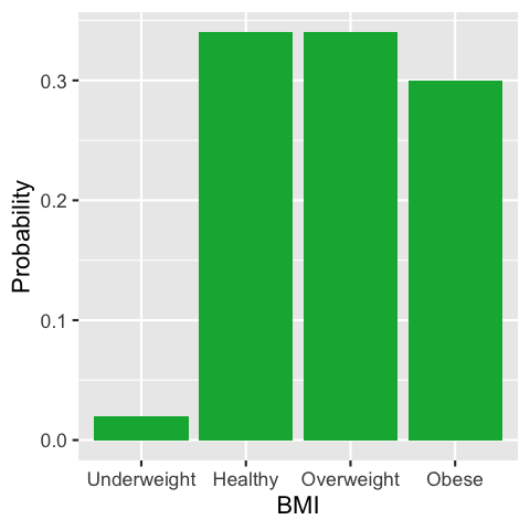
Continuous distributions
In the BMI example above, we made X into a discrete (categorical) variable by breaking it into (essentially arbitrary) ranges. In reality, BMI is a continuous, quantitative variable which can take on any positive value, not necessarily a whole number. In this situation we can no longer talk about the "probability a variable is equal to" some particular number. Why not?
Consider trying to establish if an individual's BMI is equal to 26. BMI is weight (in kilograms) divided by the square of height (in meters). In theory, we could measure both of these quantities to an arbitrary degree of precision. So while an individual might have a BMI of 26 when rounded to the nearest whole number, and maybe even 26.0 when rounded to one decimal place, if we increase the precision enough we will find some difference, no matter how small, between the individual's BMI and the value 26. Consequently, the probability their BMI is exactly equal to 26 is mathematically zero. The same is true for any other value to which we want to compare their BMI!
Instead, we can talk about the probability that an individual's BMI is in some range of values. In this case, the graph of the distribution is interpreted as having an area in any given range equal to the probability the variable lies in that range.
We've already seen that the probability the BMI lies in the range 25 to 30 is 0.34 (i.e. 34%), so the distribution
of BMI as a continuous variable might look like:
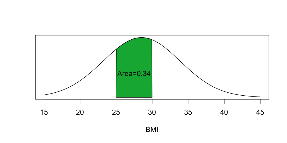
Thinking of the probability that the BMI lies in a range, instead of being exactly equal to some number, solves the problem of being equal, given a specific precision. For example, the probability that an individual's BMI is equal to 26 when rounded to the nearest whole number is equivalent to the probability their BMI lies in the range 25.5 < BMI < 26.5. And similarly, the probability it is equal to 26.0 to one decimal place is the probability it lies in the range 25.95 < BMI < 26.05.
Shapes of distributions
Mode


Symmetry
A distribution is symmetrical if there is some vertical line so that the distribution to the left of the vertical line mirrors the distribution to the right of the vertical line. In a symmetric distribution, the position of the vertical line of symmetry is equal to both the mean and the median of the distribution.
Skewed distributions
A distribution that is not symmetric is called skewed. If the left tail of the graph is longer, then the distribution is called left-tailed, or left skewed, or negatively skewed. If the right tail of the graph is longer, then the distribution is called right-tailed, or right skewed, or positively skewed.
It is a general rule of thumb (though not true for every possible distribution) that in a right-skewed distribution,
the mean is to the right of the median, which in turn is to the right of the mode. Generally, in a left-skewed
distribution, the mean is to the left of the median, which is to the left of the mode.

Did I understand this?
- The BMI of all adults in the US is a right-skewed, unimodal distribution.
(It is right-skewed because there are more overweight people than underweight, and
those who are overweight span a wider range of BMIs than those who are underweight.)
Which of the following is most likely?
-
The mean BMI and the median BMI are both equal to 24.
-
The mean BMI is 24 and the median BMI is 25.
-
The mean BMI is 25 and the median BMI is 24.
-
The mean BMI is 21 and the median BMI is 22.
-
The mean BMI and the median BMI are both equal to 22.
Incorrect
In a right-skewed distribution, the mean is typically larger than the median.
Correct!
In a right-skewed distribution, the mean is typically larger than the median.
This answer is the only answer consistent with that.
- What properties would you expect of the distribution of heights of all adult women in the US?
-
Unimodal and highly right-skewed
-
Unimodal and approximately symmetric
-
Unimodal and highly left skewed
-
Bimodal and approximately symmetric
-
Bimodal and highly right-skewed
Incorrect
The mean height of a woman in the USis around 66 inches (5'6).
Women are approximately equally likely to be taller or shorter than this mean,
with values becoming less likely the further you get from the mean.
Correct!
The mean height of a woman in the US is around 66 inches (5'6).
Women are approximately equally likely to be taller or shorter than this mean,
so the distribution is symmetric.
Values becoming less likely the further you get from the mean, so there are no additional
peaks in the distribution.
- What properties would you expect of the distribution of heights of all adults (men and women) in the US?
-
Unimodal and highly right-skewed
-
Unimodal and approximately symmetric
-
Unimodal and highly left skewed
-
Bimodal and approximately symmetric
-
Bimodal and highly right-skewed
Incorrect
The mean height of a woman in the US is around 66 inches (5'6),
and the mean height of a man is around 69 inches (5'9).
Both women and men are approximately equally likely to be taller or shorter than the
respective means,
with values becoming less likely the further you get from the mean.
Correct!
The mean height of a woman in the US is around 66 inches (5'6),
and the mean height of a man is around 69 inches (5'9).
Since there are two distinct means, and the number of men and
women are approximately equal, there are likely to be two peaks in the
distribution, so it is likely to be bimodal.
Both women and men are approximately equally likely to be taller or shorter than the
respective means,
with values becoming less likely the further you get from the mean, so
the distribution will be approximately symmetric.
- The mean BMI and the median BMI are both equal to 24.
- The mean BMI is 24 and the median BMI is 25.
- The mean BMI is 25 and the median BMI is 24.
- The mean BMI is 21 and the median BMI is 22.
- The mean BMI and the median BMI are both equal to 22.
- Unimodal and highly right-skewed
- Unimodal and approximately symmetric
- Unimodal and highly left skewed
- Bimodal and approximately symmetric
- Bimodal and highly right-skewed
- Unimodal and highly right-skewed
- Unimodal and approximately symmetric
- Unimodal and highly left skewed
- Bimodal and approximately symmetric
- Bimodal and highly right-skewed