BMR 617: Statistical Techniques for the Biomedical Sciences

Principles for presenting statistical ananlyses

Statistical analyses are an important part of any experiment or study. The same principles that apply to other parts of the scientific process also apply to the statistical analyses. In particular:

• Statistical analyses should be valid, and in a publication must be verifiable. This means the appropriate analyses should be used, and sufficient detail should be provided so that a reader or reviewer can verify that the appropriate analyses have been performed.
• Analyses should be reproducible. In the context of the statistical analyses, this means that another scientist should be able to start from the same data and produce the same results of the analysis.

Structure of a journal article

Journal articles are typically presented in three main sections:

• Methods
• Results
• Discussion
When presenting the statistics, the methods section should contain sufficient detail on the statistical methods used that another scientist, given the raw data, would be able to reproduce the results. At a minimum, this means you should include:
• What statistical tests were performed for each analysis?
• What software and version of the software were used to perform the analyses?

In an ideal world, all raw data would be available to reviewers and readers, and the reviewer and/or reader would be able to reproduce the results and visualizations that appear in the journal article. While this is rarely acheived, some current steps are moving this closer to reality. For example, the National Institutes of Health recently released a new requirement for all NIH funded research to have a data management and sharing plan, in which all experimental data are shared in public repositories. If this is combined with performing analyses either using software that supports scripting (such as R), or using software that can generate a record of what was done ("cookie trails"), then scripts or records can be included with the raw data or with supplemental data to the publication.

The results section should include the results of the statistical analyses performed. This can be in the form of graphs, text, or both. In either case, the results of each statistical test should include:

• The effect size. This is the difference in means between two groups (for a t-test, or post-hoc tests for an ANOVA), or the relative risk or odds ratio (for comparing proportions), or a correlation coefficient, \(R^2\) value, or parameter estimate for a linear regression.
• Confidence intervals for the effect sizes. State the level of confidence chosen (this will usually be 95%).
• The p-value. Avoid simply characterizing the p-value as "significant" or "not significant"; always give an actual value. Include all p-values, even those not considered significant.
Always give sufficient information to make it clear what the results mean. For example, in an ANOVA, make sure it is clear which is the "reference" level. When providing an odds ratio or relative risk, make sure it is clear which odds (or risk) are calculated, and which experimental condition is used for the numerator and denominator of the ratio.

Do not try to interpret the results in the results section. Biological implications of the results obtained should be in the discussion section.

Example

Let's work through our Cholesterol example from the mouse data. Here is the R code for performing a two-way ANOVA and plotting a graph:

	
library(tidyverse)
met <- read_csv("https://denvirlab.marshall.edu/BMR617-2023/data/TH-B6-metabolic.csv") %>%
  separate(MouseID, into=c("Strain", "Diet", "ID"), sep='-')

aov.full <- aov(Cholesterol ~ Strain * Diet, data = met)
aov.full$coefficients
confint(aov.full)
summary(aov.full)

png(filename = "figure1.png", width=8*960, height = 8*480, res=8*72)
ggplot(met, aes(x=Strain, y=Cholesterol, fill=Diet)) +
  geom_boxplot(outlier.shape = NA) + 
  geom_point(position=position_jitterdodge(jitter.width = 0.1, dodge.width = 0.75)) +
  xlab("Cholesterol Level (mg/dl)") +
  ggtitle("Cholesterol Level by Mouse Strain and Diet")
dev.off()

sessionInfo()
	
	

Methods

For the methods, we need to state the analysis that was performed. What we actually performed was a two-way ANOVA with interaction. That should be the first thing we state. The sessionInfo() command gives us details of the version of R and any packages we are using. The following should be considered the minimum information that is required for a journal article.

Statistical methods

The effect of mouse strain and diet on cholesterol level was assessed using a two-way ANOVA with interaction.

All statistical analyses were performed using the statistical computing environment R [1], version 4.2.1, with the "tidyverse" package [2], version 1.3.2.

To get the correct references, we can use the citation() function:

citation()
citation("tidyverse")
	

So here our references would be
1. R Core Team (2020). R: A language and environment for statistical computing. R Foundation for Statistical Computing, Vienna, Austria. URL https://www.R-project.org/.
2. Wickham et al., (2019). Welcome to the tidyverse. Journal of Open Source Software, 4(43), 1686, https://doi.org/10.21105/joss.01686

For more robustness and reproducibility, we could place the CSV file with the raw data in a public data repository, and include the R script, either in the same repository (if permitted), in a software repository such as GitHub, or as a supplemental file for the manuscript.

Results

The R code above generates the following output:

> library(tidyverse)
> met <- read_csv("https://denvirlab.marshall.edu/BMR617-2022/data/TH-B6-metabolic.csv") %>%
+   separate(MouseID, into=c("Strain", "Diet", "ID"), sep='-')
Rows: 29 Columns: 7                                                                                                         
── Column specification ──────────────────────────────────────────────────────────────────────────────────────────────────────
Delimiter: ","
chr (1): MouseID
dbl (6): BodyWeight, Insulin, TG, Cholesterol, Glucose, FatMass

ℹ Use `spec()` to retrieve the full column specification for this data.
ℹ Specify the column types or set `show_col_types = FALSE` to quiet this message.
> 
> aov.full <- aov(Cholesterol ~ Strain * Diet, data = met)
> aov.full$coefficients
    (Intercept)        StrainTH          DietHF          DietLF StrainTH:DietHF StrainTH:DietLF 
      42.945000       58.290000       72.140998       38.783333        8.934004        7.221669 
> confint(aov.full)
                      2.5 %    97.5 %
(Intercept)      13.1490209  72.74098
StrainTH         19.8235566  96.75644
DietHF           32.1654973 112.11650
DietLF            0.3168892  77.24978
StrainTH:DietHF -49.1490529  67.01706
StrainTH:DietLF -45.5208619  59.96420
> summary(aov.full)
            Df Sum Sq Mean Sq F value   Pr(>F)    
Strain       1  19984   19984  24.082 5.87e-05 ***
Diet         2  25773   12887  15.529 5.40e-05 ***
Strain:Diet  2    102      51   0.062     0.94    
Residuals   23  19086     830                     
---
Signif. codes:  0 ‘***’ 0.001 ‘**’ 0.01 ‘*’ 0.05 ‘.’ 0.1 ‘ ’ 1
> 
> png(filename = "figure1.png", width=8*960, height = 8*480, res=8*72)
> ggplot(met, aes(x=Strain, y=Cholesterol, fill=Diet)) +
+   geom_boxplot(outlier.shape = NA) + 
+   geom_point(position=position_jitterdodge(jitter.width = 0.1, dodge.width = 0.75)) +
+   xlab("Cholesterol Level (mg/dl)") +
+   ggtitle("Cholesterol Level by Mouse Strain and Diet")
> dev.off()
RStudioGD 
        2 
> 
> sessionInfo()
R version 4.2.1 (2022-06-23)
Platform: x86_64-apple-darwin17.0 (64-bit)
Running under: macOS Monterey 12.3

Matrix products: default
LAPACK: /Library/Frameworks/R.framework/Versions/4.2/Resources/lib/libRlapack.dylib

locale:
[1] en_US.UTF-8/en_US.UTF-8/en_US.UTF-8/C/en_US.UTF-8/en_US.UTF-8

attached base packages:
[1] stats     graphics  grDevices utils     datasets  methods   base     

other attached packages:
[1] forcats_0.5.1   stringr_1.4.0   dplyr_1.0.9     purrr_0.3.4    
[5] readr_2.1.2     tidyr_1.2.0     tibble_3.1.8    ggplot2_3.3.6  
[9] tidyverse_1.3.2

loaded via a namespace (and not attached):
 [1] tidyselect_1.1.2    haven_2.5.0         gargle_1.2.0       
 [4] colorspace_2.0-3    vctrs_0.4.1         generics_0.1.3     
 [7] utf8_1.2.2          rlang_1.0.4         pillar_1.8.0       
[10] glue_1.6.2          withr_2.5.0         DBI_1.1.3          
[13] bit64_4.0.5         dbplyr_2.2.1        modelr_0.1.8       
[16] readxl_1.4.0        lifecycle_1.0.1     munsell_0.5.0      
[19] gtable_0.3.0        cellranger_1.1.0    rvest_1.0.2        
[22] labeling_0.4.2      tzdb_0.3.0          parallel_4.2.1     
[25] curl_4.3.2          fansi_1.0.3         broom_1.0.0        
[28] scales_1.2.0        backports_1.4.1     googlesheets4_1.0.0
[31] vroom_1.5.7         jsonlite_1.8.0      farver_2.1.1       
[34] fs_1.5.2            bit_4.0.4           digest_0.6.29      
[37] hms_1.1.1           stringi_1.7.8       grid_4.2.1         
[40] cli_3.6.0           tools_4.2.1         magrittr_2.0.3     
[43] crayon_1.5.1        pkgconfig_2.0.3     ellipsis_0.3.2     
[46] xml2_1.3.3          reprex_2.0.1        googledrive_2.0.0  
[49] lubridate_1.8.0     assertthat_0.2.1    httr_1.4.3         
[52] rstudioapi_0.13     R6_2.5.1            compiler_4.2.1  
	

The key points here are:

• Strain has an effect on Cholesterol level, with TH mice having a higher cholesterol level than B6 mice.
• Diet has an effect on Cholesterol level, with mice fed the LF diet having a higher Cholesterol level than mice fed the Chow diet, and mice fed the HF diet having a higher Cholesterol level than the mice fed the Chow diet.
• There is no evidence of an interaction between Strain and Diet on the Cholesterol level.
• All these effects can be quantified, and confidence levels computed.

The R code above generates a PNG graphics file: 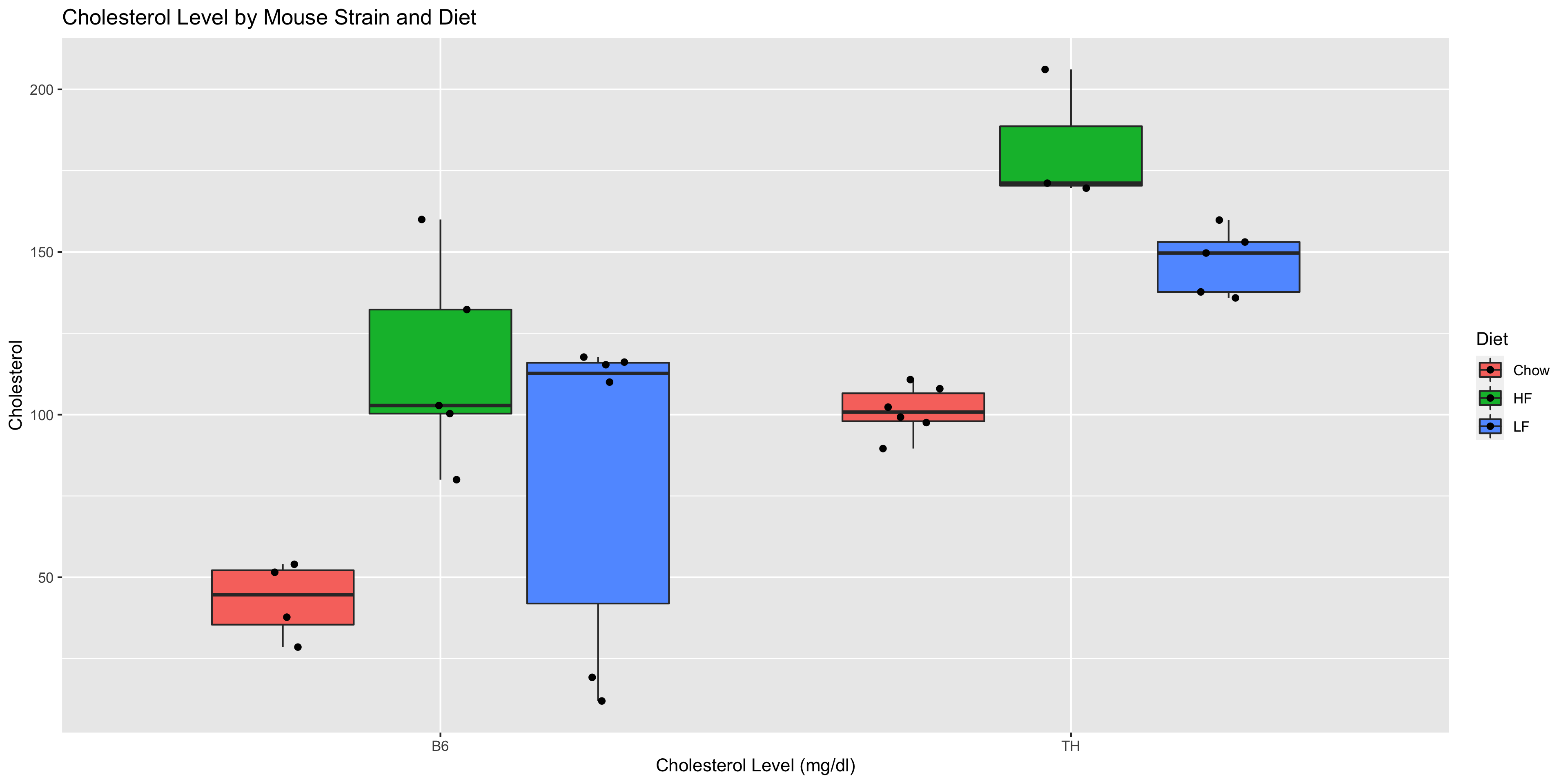The figure should have a legend that states simply what is represented.

Cholesterol levels for C57BL/6 ("B6") and TALLYHO ("TH") mice fed Chow, high-fat ("HF"), or Low-fat ("LF") diets from weaning until 16 weeks of age. Box plots indicate median (solid line), interquartile range (box) and range. Points indicate individual values for replicates (n=3-6)

If you choose to use bar charts, then the figure legend should state what the error bars represent.

Presenting results in the narrative

We can summarize the results above in a narrative. Each statement should be backed with quantities and confidence intervals. We should also include p-values. The following provides a concise, precise summary of the results:

Both Strain (\(p=5.87\times10^{-5}\)) and Diet (\(p=5.40\times10^{-5}\)) showed an effect on Cholesterol levels. The mean Cholesterol level for the control B6 mice fed the Chow diet was 42.95mg/dl (95% CI [13.15, 72.74]). TH mice had Cholesterol levels an average of 58.28mg/dl (95% CI [19.82, 96.76]) higher than B6 mice. Mice fed the Low-fat, high-calorie ("LF") diet had cholesterol levels an average of 38.73mg/dl (95% CI [0.32, 77.25]) higher than those fed the Chow diet, while mice fed the High-Fat ("HF") diet had Cholesterol levels an average of 72.14mg/dl (95% CI [32.17, 112.12]) higher that those fed Chow. There was no evidence of an interaction between mouse Strain and Diet (p=0.94).
Note here that we include exact p-values (not just p<0.05 or p>0.05) and include the p-values for non-significant results. We also include confidence intervals each time we refer to an estimate.

Wrangling the results to a table

To create a table with the results, we need to combine different parts of the output from R into a single table. We can do this with a bit of effort and some data wrangling in R. We'd like to create a table with the parameters, estimates, and 95% confidence intervals.

The estimates are contained in aov.full$coefficients, as a named list.

The 95% confidence intervals are contained in confint(aov.full), which is a matrix. The row names of the matrix contain the parameter names.

We can start by converting the matrix containing the confidence intervals to a tidyverse data table:

resultsTable <- as_tibble(confint(aov.full), rownames="Parameter")
	

Now let's add a column for the estimate. We can turn the list aov.full$coeffcients into another data table, and bind its columns (cbind(...)) with our existing table:

resultsTable <- cbind(resultsTable, tibble(Estimate = aov.full$coefficients))
	

Let's tidy this up a bit. We can round the numerical columns to two digits, and combine the two columns representing the confidence interval into a single column:

resultsTable <- resultsTable %>%
  mutate(`2.5 %` = round(`2.5 %`, digits = 2),
         `97.5 %` = round(`97.5 %`, digits = 2),
         Estimate = round(Estimate, digits = 2)) %>%
  mutate(`95% Confidence Interval`=paste0("[", `2.5 %`, ", ", `97.5 %`, "]"))
	

and finally we can just select the columns we need:

resultsTable <- resultsTable %>%
  select(Parameter, Estimate, `95% Confidence Interval`)
  	

We can save this as a CSV file and paste it into a Word document. The final table looks like:

Parameter	Estimate	95% Confidence Interval
(Intercept)	42.95	[13.15, 72.74]
StrainTH	58.29	[19.82, 96.76]
DietHF	72.14	[32.17, 112.12]
DietLF	38.78	[0.32, 77.25]
StrainTH:DietHF	8.93	[-49.15, 67.02]
StrainTH:DietLF	7.22	[-45.52, 59.96]

Outputting graphics

The code above generates the following graph:



The basic code structure is

png("ImageFilename.png", ...)
# Graphics commands
dev.off()
	

This will create an image file with the name ImageFilename.png. Any graphics commands will be written to an off-screen "graphics device", and when dev.off() ("device off") is called, all the graphics will be written to that file, and the file will be closed.

Controlling the image quality

Computer graphics are represented by an array of individual dots, called pixels. Each pixel is a small rectangle in one solid color. Our aim is to generate images that look good on a screen and in print. On a screen, a user might zoom in to see more detail.

When we create the png file, we can specify the size in pixels. The default size is 480 by 480, which is not a very high resolution.

png("lowResChol.png", width=480, height=480)
ggplot(met, aes(x=Strain, y=Cholesterol, fill=Diet)) +
  geom_boxplot(outlier.shape = NA) + 
  geom_point(position=position_jitterdodge(jitter.width = 0.1, dodge.width = 0.75)) +
  ylab("Cholesterol Level (mg/dl)") +
  ggtitle("Cholesterol Level by Mouse Strain and Diet")
dev.off()

If we increase the image size, we get a much higher-quality images:

png("hiResChol.png", width=8*480, height=8*480)
ggplot(met, aes(x=Strain, y=Cholesterol, fill=Diet)) +
  geom_boxplot(outlier.shape = NA) + 
  geom_point(position=position_jitterdodge(jitter.width = 0.1, dodge.width = 0.75)) +
  ylab("Cholesterol Level (mg/dl)") +
  ggtitle("Cholesterol Level by Mouse Strain and Diet")
dev.off()

The problem now is that the text is too small to see. Text size is not measured in pixels, but in point size. Usually, there are 72 points to an inch, so these units are in "print size", not "image size". We can control this with the res parameter, which scales the point size, and effectively determines the number of points per pixel.

png("hiResChol.png", width=8*480, height=8*480, res=8*72)
ggplot(met, aes(x=Strain, y=Cholesterol, fill=Diet)) +
  geom_boxplot(outlier.shape = NA) + 
  geom_point(position=position_jitterdodge(jitter.width = 0.1, dodge.width = 0.75)) +
  ylab("Cholesterol Level (mg/dl)") +
  ggtitle("Cholesterol Level by Mouse Strain and Diet")
dev.off()