BMR 617 - Linear Regression

Introduction

This is a very brief introduction to the idea of linear models. A large proportion of statistics, including virtually everything we've seen so far, can be seen from a unifying perspective of linear models.

Statistical Models

A statistical model is a mathematical function that predicts the value of a response variable from the values of the explanatory variables. The model depends on parameters. These parameters are properties of the population; they are fixed (their values do not depend on the data we collect) but are unknown. We collect data (our sample), and use the data to estimate the values of the parameters.

Linear regression is an example of a statistical model. With the COVID-19 case data, we modeled the log of the number of cases as a linear function of time: \[\log(y) = a + b\times t\] where \(y\) is the number of cases, \(a\) the log of the number of cases at the first day of measurement, and \(b\) the increase in the log of the number of cases per day.

In multiple linear regression, we modeled the median house price of homes in Boston suburbs as a function of 12 social and economic variables associated with those suburbs. The parameters were the increases in median house price per unit increase in each of the variables.

As an way to see how a lot of what we've looked at can be viewed from the perspective of linear models, let's look at a t-test. For reasons we'll explain later, we'll use a t-test that assumes equal variance between the two groups:


library(tidyverse)
met <- read_csv('https://denvirlab.marshall.edu/BMR617-2023/data/TH-B6-metabolic.csv') %>%
  separate(MouseID, sep="-", into=c("Strain", "Diet", "ID")) %>%
  mutate(Strain = as.factor(Strain), Diet = as.factor(Diet))

met.chow <- met %>% filter(Diet == "Chow")

t.test(Cholesterol ~ Strain, data = met.chow, var.equal = TRUE)

Linear regression, as we've seen it so far, requires the response variable and the explanatory variable to be quantitative. Here the explanatory variable, Strain, is categorical. So let's define a "dummy variable" (we'll call it CodedStrain which takes the value 0 for B6 mice and 1 for TH mice:


met.chow <- met.chow %>% mutate(CodedStrain = ifelse(Strain=="B6", 0, 1))

Remember mutate can be used to add a new column to a data table. Here we have mutate(CodedStrain = ...), and since CodedStrain doesn't match any existing columns, we are creating a new column called CodedStrain.

The function ifelse takes three arguments. The first is a logical (i.e. something that can either be TRUE or FALSE). The second is the value to use if the first argument is TRUE, and the third is the value to use if the first argument is FALSE. So this will be 0 if the Strain is B6, and 1 otherwise. You can check this by clicking on met.chow in the "Environment" tab.

Now lets fit a linear regression and examine it:


summary(lm(Cholesterol ~ CodedStrain, data = met.chow))

From the t-test, what is the mean of each group? What is the difference in means?

From the linear regression, what is the estimated intercept? What is the estimated slope?

What do you notice?

What about the p-values for the t-test and the linear regression? What do you notice?

Can you explain these findings?

An equal-variance t-test is a linear regression

To understand why these are the same, consider plotting Cholesterol against the CodedStrain:


ggplot(met.chow, aes(x=CodedStrain, y=Cholesterol)) + geom_point()

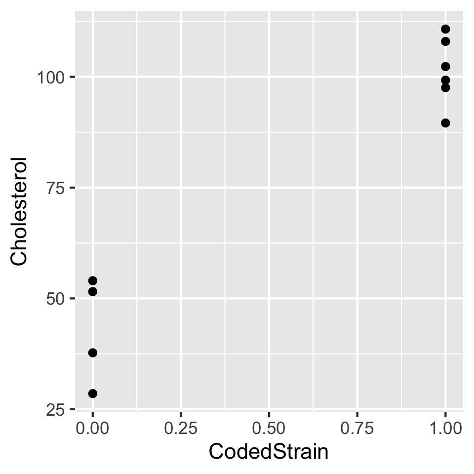
Let's imagine trying to find the "line of best fit" through these points. The intercept is the y-value where the line passes x=0. This means it's the line that passes through the points for the B6 mice, in the column at x=0.

Once we've found an intercept, choosing the slope will determine where the line passes through x=1, i.e. where the line passes through the points for the TH mice, in the column on the right.

We have to choose this line to minimise the sum of the squares of the vertical distances of each point from the line. It's not too hard to see that the best choice for the line passes through the mean of both sets of points.

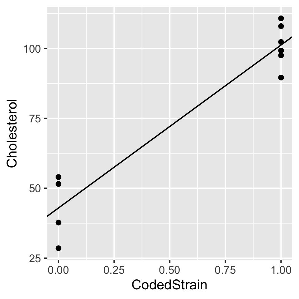
Now the intercept is just the y-value on the line when x=0, which is the mean for the B6 mice.

The slope is the difference in y-value between any two points divided by the difference in x-value between the same two points. So it's the difference in means between the two groups divided by 1.

The p-value for the linear regression is calculated for the null hypothesis that the slope is zero, which is the null hypothesis that the means are equal. This is the same null hypothesis that we use for the t-test.

Finally, recall that one of our assumptions for linear regression is that the distribution of residuals (distances of the points from the line) is the same for all x-values. Here, since there are only two x-values, this means that the variance in y is the same at x=0 as it is at x=1. This is the same as saying that the variance in one group is the same as the variance in the other, which is why we use an "equal variances" t-test.

There's actually no need to create the numerical variable. The lm function that creates the fit to the linear model will (silently) do that for us if we use a factor as one of the variables in the model:


summary(lm(Cholesterol ~ Strain, data = met.chow))

You can actually see what the model will use behind the scenes using the contrasts function:


contrasts(met.chow$Strain)

The output is


   TH
B6  0
TH  1

This indicates it introduces one "dummy variable" with value TH (first, and only, column in the output). The value of the variable is 0 if Strain=="B6" (first row in the output) and 1 if Strain=="TH" (second row in the output).

Paired t-tests and Linear Models

Let's look again at our Western Blot data from the Renal Cancer project:


rwd <- read_csv("https://denvirlab.marshall.edu/BMR617-2023/data/RenalWesternData.csv")

and focus just on the data for the protein SGK1:


sgk1 <- filter(rwd, Protein=="SGK1")

Fit the following model, and let's think about what the parameter for TissueType represents:


sgk1.pt.tt <- lm(Expression ~ TissueType + Patient, data=sgk1)
summary(sgk1.pt.tt)

Each parameter is the estimated effect of that parameter, if the other variables are held constant. So the parameter TissueTypeTumor represents the effect on SGK1 expression of the tumor tissue type, if the patient is held constant. I.e. it's the difference between the expression in the tissue types on a per-patient basis. Alternatively, we can think of this as the effect of the tissue type, correcting for the difference between patients. Note the effect is an increase of 5,388,495 (again, the units are somewhat arbitrary), and the p-value is 0.0329.

Recall how we ran a paired t-test for these data:


t.test(Expression ~ TissueType, paired=T, data=sgk1)

What is the mean difference? What is the p-value?

So a paired t-test is just a linear regression in which we "correct for the experimental unit" (in this case the "experimental unit" is the patient).

Dummy variables with more than two levels

How does a linear model work if we use an categorial explanatory variable with more than two levels? Let's use our example of a one-way ANOVA, where we looked at the effect of diet on B6 mice.


met.b6 <- filter(met, Strain=="B6")

It's tempting to think this would use a single dummy variable for Diet, and assign three different values for the diets, for example, 0 for Chow, 1 for LF, and 2 for HF. However, this is problematic, because it assigns a scale that doesn't exist to the variable. In this case, it makes the "difference between LF and Chow" the same as the "difference between HF and LF". Since categorical variables do not have a notion of scale, there is no way to do this with a single variable in a way that works.

We can use the contrasts function to see what actually happens:


contrasts(met.b6)

This results in:


     HF LF
Chow  0  0
HF    1  0
LF    0  1

Here, two dummy variables are created (there are two columns); HF and LF. The variable HF takes the value 1 if Diet=="HF" and 0 otherwise. The variable LF takes the value 1 if Diet=="LF", and 0 otherwise. So mice fed Chow are coded (0,0), mice fed HF are coded (1,0), and mice fed LF are coded (0,1).

Let's see what the linear model gives:


fit.diet <- lm(Cholesterol ~ Diet, data=met.b6)
fit.diet
summary(fit.diet)

Compare this to the ANOVA:


aov(Cholesterol ~ Diet, data=met.b6)

It is less clear in this case, but the two tests are essentially the same (the overall p-value is identical). They present the information in a different way, because they are designed to answer different questions.

The ANOVA is asking if there is a relationship between the Cholesterol variable and the Diet variable
The linear model is asking how you can predict the value of the Cholesterol variable, given the Diet

Summary

Many of the statistical tests we've seen so far can be viewed from the perspective of linear models.
- Even Chi-squared and Fisher exact tests can be seen this way, though the treatment of this is more advanced, using something called "generalized linear models".
Linear models can be used as hypothesis tests, asking if each explanatory variable has an effect on the response variable if the other explanatory variables are kept constant
- This is sometimes called "correcting for the other variables"
Linear models can be used to predict values of the response variable.
It is sometimes useful (and it's valid) to perform both (e.g. run an ANOVA and a linear model) to see different interpretations of the same analysis.

Experiment with using lm on the two-way ANOVA and the two-way ANOVA with interactions.