BMR 617: Probability and Bayes' Theorem
Probability
Probability is the mathematical formulation of likelihood. It describes the likelihood of events occurring.
Probability can be divided into two different approaches:
- Theoretical probability
- Deduce the likelihood of events from logical reasoning given certain assumptions.
- Empirical (observational) probability
- Deduce the likelihood of events from observing a large number of outcomes
In our context, we are interested in the study and interpretation of biomedical data. We almost always make observations and work with data from a sample, and want to make inferences about how well that sample represents a wider population.
- E.g. work with data from a large clinical study, and make inferences about the whole population from which the study subjects are drawn.
- Or perform a lab experiment with a small number of replicates, and make inferences about what is inherent to the experiment and what is due to random effects.
- We'll explore these ideas more in the next few classes, but the inferences we make in these examples are deduced using probability theory.
Notation for probabilities
Given an event, which we denote \(A\), the probability of \(A\) occurring is written \(P(A)\).
Since probabilities are between 0 and 1, \[0\leq P(A) \leq 1\]
\(P(A)=0\) means \(A\) is certain not to happen; \(P(A)=1\) means \(A\) is certain to happen. \(P(A)=0.5\) means \(A\) is equally likely to happen or not happen.
We can think of \(P\) as a function from the set of all possible distinct outcomes (called the sample space) to the set of real numbers between 0 and 1 (inclusive): \[P:S\to[0,1]\] The sum of the probabilities of all possible outcomes is 1, which mathematically is written \[\sum_{A\in S}P(A)=1\]
Example
This simplest example is tossing a (fair) coin. The possible outcomes are heads (H) or tails (T), so \[S=\{H,T\}\] The probabilities of both \(H\) and \(T\) are the same, and must sum to 1, so \[P(H)=P(T)=\frac12\]Combining Probabilities
To motivate this section, think about throwing a fair, six-sided die. The sample space (possible outcomes) is \[S=\{1,2,3,4,5,6\}\] and \(P(A)=\frac{1}{6}\) for each \(A\in S\).
What is the probability that a throw of the die gives a number greater than 4?
Why?
What is the probability of an odd number from a single throw?
The addition rule
In probabilistic language, if \(A\) and \(B\) are events, the event “A or B” refers to at least one of \(A\) or \(B\) occurring- I.e. \(A\) happens, or \(B\) happens, or both happen
The addition rule states that
If \(A\) and \(B\) are disjoint events, \[P(A \operatorname{or} B) = P(A) + P(B)\]Here "disjoint events" means that \(A\) and \(B\) cannot both happen together.
For the die example, \[P(X > 4) = P(5\operatorname{or}6)=P(5)+P(6)=\frac16+\frac16=\frac13\] because 5 and 6 are events that cannot both happen together.
Similarly, \[P(\operatorname{odd})=P(1\operatorname{or} 3\operatorname{or} 5)=\frac12\]
Events that are not disjoint
What is the probability of getting an odd numbered throw or a throw greater than 4 on a single roll of the die?
Are these two events disjoint?
We can visualize these with a Venn Diagram: here A is the event of an
odd numbered throw and B is the event of a throw greater than 4.
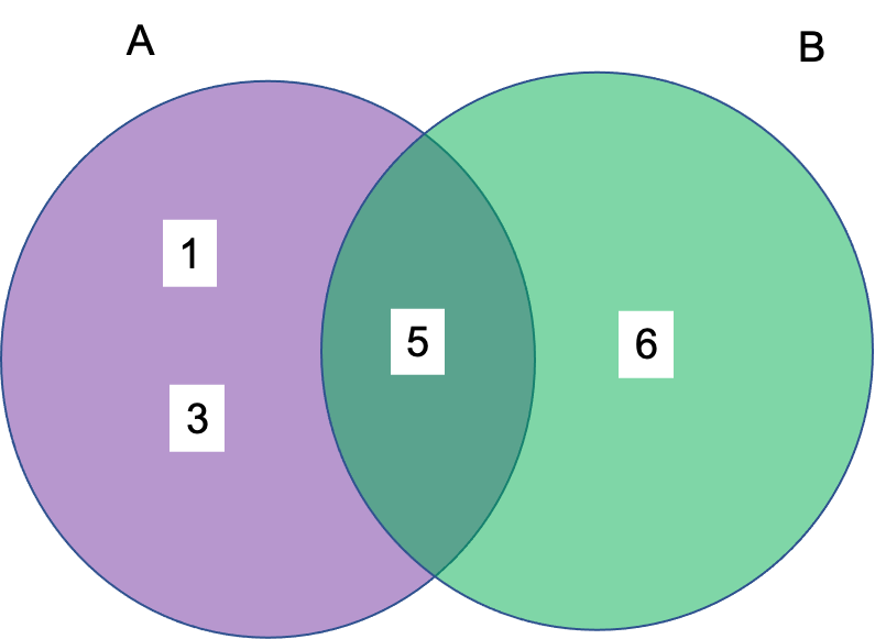
Note that \(P(A)=\frac36\) and \(P(B)=\frac26\).
The general addition rule
If we try to use the addition rule in the previous example, we get the wrong result: \[P(A)+P(B)=\frac56\] but \[P(1\operatorname{or} 3\operatorname{or} 5\operatorname{or} 6)=\frac46=\frac23\]
The problem is that we "count 5 twice", because it is part of both event \(A\) and event \(B\).
The general addition rule contains a fix for this: \[P(A\operatorname{or}B)=P(A)+P(B)-P(A\operatorname{and}B)\]
The multiplication rule
We say that two events \(A\) and \(B\) are independent if \(P(B)\) does not depend on whether or not \(A\) occurs
If \(A\) is the event of a throw greater than 4, and \(B\) is the event of an odd numbered throw, are these independent?
If \(A\) is the event of a throw greater than 3, and \(B\) is the event of an odd numbered throw, are these independent?
We'll revisit these questions later.
The multiplication rule states that if \(A\) and \(B\) are independent, then \[P(A\operatorname{and}B)=P(A)\times P(B)\]
Conditional Probability
We define conditional probability as the probability of an event \(A\) happening, given that an event \(B\) has happened, and we denote this as \(P(A|B)\). This probability is defined as \[P(A|B)=\frac{P(A\operatorname{and} B)}{P(B)}\]
Conditional Probability: Motivation
To motivate the definition of conditional probability, consider the example where \(A\) is the event that our die throw is odd, and \(B\) is the event that our die throw is greater than 3. We want to know the probability the throw is odd, given that it’s greater than 3.
Intuitively, if it’s greater than 3, there are three equal possibilities (4, 5, and 6). One of these is odd, so the probability should be 1/3.
Note here we divide the number of occurrences (1) of both events by the number of occurrences (3) of the “given” event
Equivalently, we can divide the probability of both events (\(\frac16\)) by the probability of the ”given” event (\(\frac36\), or \(\frac12\)).
Formally, \[P(A|B)=\frac{P(A\operatorname{and}B)}{P(B)}=\frac{1/6}{1/2}=\frac13\]
Independence, revisited
We can now formally define independence:
Events \(A\) and \(B\) are called independent if \[P(A|B)=P(A)\] I.e. the probability of \(A\) given that \(B\) has occurred is the same as the probability of \(A\). Or in other words, \(B\) happening or not happening does not change the probability of \(A\).
Let's revisit these two questions:
If \(A\) is the event of a throw greater than 4, and \(B\) is the event of an odd numbered throw, are these independent?
If \(A\) is the event of a throw greater than 3, and \(B\) is the event of an odd numbered throw, are these independent?
Bayes Theorem
Bayes theorem is one of the fundamental theorems of probability.
Remember we have \[P(A|B)=\frac{P(A\operatorname{and}B)}{P(B)}\] which we could just write as \[P(A\operatorname{and}B)=P(A|B)\times P(B)\]
Let's think about \(P(B|A)\), the probability of \(B\) given that \(A\) has happened. By definition, this must be \[P(B|A)=\frac{P(B\operatorname{and}A)}{P(A)}\] which we can write as \[P(B\operatorname{and}A)=P(B|A)\times P(A)\] However, the event "A and B" is the same as the event "B and A", so \[P(A|B)\times P(B)= P(B|A)\times P(A)\] which we can rewrite in the usual form of Bayes Theorem: \[P(B|A)=\frac{P(A|B)\times P(B)}{P(A)}\] This gives us a way to find the probability of \(B\) given \(A\) in terms of the probability of \(A\) given \(B\) (if we know the probabilities of each).
Example: Twins
Twins can occur in two different ways:
- A single zygote created during fertilization divides into two embryos. This creates “monozygotic” twins.
- Two zygotes are created during fertilization (from two sperm and two egg cells), and both go on to form embryos. This creates “dizygotic” twins.
Note that in the first case, the two twins have exactly the same genetics. These are known colloquially as “identical twins”.
n the second case, the zygotes come from different rearrangements of the parental genomes, so they are genetically distinct. These are known colloquially as “fraternal twins”.
Bayes Theorem: Twins
Suppose that, in a given population, 25% of all twins are monozygotic (identical) twins, and consider the following scenario.
A pregnant woman visits her OB/GYN. Through listening with a stethoscope, the nurse determines she is pregnant with twins.
- At this point, with the knowledge we have, the probability these are identical twins is 0.25.
- Given this new information, is the probability the twins are identical still 0.25? If not, is it more, or less, than 0.25?
We can approach this question using Bayes Theorem.
Applying Bayes Theorem: Step 1
Let \(M\) be the event that the twins are monozygotic, and let \(GG\) be the event that the twins are both girls. We know that the event \(GG\) has occurred, and want to know the probability of event \(M\) given this information. I.e. we want to know \[P(M|GG)\] By Bayes Theorem: \[P(M|GG) = \frac{P(GG|M)\times P(M)}{P(GG)}\]
The hardest part of this is \(P(GG)\).
There are two ways \(GG\) can happen: either we have two monozygotic girls, or two dizygotic girls. Since these are disjoint, \[P(GG)=P(GG\operatorname{and}M)+P(GG\operatorname{and not}M)\]
For the first part of this, remember that monozygotic twins come from a single zygote. That zygote has a probability of \(\frac12\) of having two X chromosomes, so \[P(GG|M)=\frac12\] We are assuming \(P(M)=\frac14\), so \[P(GG\operatorname{and}M)=P(GG|M)\times P(M)=\frac12\times\frac14=\frac18\] On the other hand, dizygotic twins come from two different zygotes. The probability of each having two X chromosomes is 1⁄2, and these are independent, so \[P(GG|\operatorname{not} M)=\frac14\] So \[P(GG\operatorname{and}\operatorname{not}M)=P(GG|\operatorname{not}M)\times P(\operatorname{not}M) =\frac14\times\frac34=\frac3{16}\] Finally (for this step!) \[P(GG)=\frac18+\frac3{16}=\frac{5}{16}\]
Applying Bayes Theorem: Step 2
We have \[P(M|GG) = \frac{P(GG|M)\times P(M)}{P(GG)}\]
In the previous step, we computed \(P(GG)=\frac5{16}\).
In the process, we also computed \(P(GG|M)=\frac12\). So we have \[P(M|GG)=\frac{1/2 \times 1/4}{5/16}=\frac{1/8}{5/16}=\frac25\]
The probability of identical twins, given the information that both twins are girls, is \(\frac25\) (40%), which is more than our previous probability of \(\frac14\) (25%).
The additional information (two girls), which is compatible with the question we are asking (are the twins monozygous?), increases the likelihood of the question we are asking being true.
Summary
Probability gives a rigorous mathematical formulation of the idea of likelihood.
Bayes Theorem provides a framework for changing the measure of likelihood based on new information.
Formal arguments using probability are subtle and difficult. We will not need to delve in this depth very often.
Probability is used in statistics to make inferences from data. The typical approach is:
- Suppose we have a hypothesis and perform an experiment to test it. How likely would it be that we would get the data we actually saw, if our hypothesis were wrong?