BMR 617: Statistical Techniques for the Biomedical Sciences
Inference: Matched Pairs t-test (Paired t-test)
This type of t-test is used to compare two dependent means of quantitative variables. It is also called repeated-measures t-test, paired samples t-test, or matched samples t-test. Paired t-test assumes that the population standard deviation of the paired differences is unknown and will be estimated through the data.
Recall the pooled and unpooled two-sample t-tests.
We will use the following variables in this section:
H0: null hypothesis
Ha: alternative hypothesis
μ1: mean of population 1
μ2: mean of population 2
x1 and x2: computed (observed) sample means of groups 1 and 2, respectively
n1 and n2: sample sizes of groups 1 and 2, respectively
s12 and s22: computed sample variances of groups 1 and 2, respectively
sp2: computed common sample variance (estimator of the pooled variance of groups 1 and 2)
sp: computed common sample standard deviation
Classical t-test ("pooled two-sample t-test") is used when the variance of two groups being compared are equivalent.
The test statistic value t, i.e., [(sample mean difference – population mean difference)/standard error], would be
$$ {t = \frac{\bar{x_1} - \bar{x_2} - Δ_0}{\sqrt{s_p^2({\frac{1}{n_1} + \frac{1}{n_2}})}} = \frac{\bar{x_1} - \bar{x_2}}{s_p\sqrt{{\frac{1}{n_1} + \frac{1}{n_2}}}}} $$
where μ1-μ2 is replaced by the null value Δ0, which is equal to zero.
H0: μ1 = μ2 or μ1 - μ2 = 0
Ha: μ1 ≠ μ2 or μ1 - μ2 ≠ 0
H0: μ1 ≤ μ2 or μ1 - μ2 ≤ 0
Ha: μ1 > μ2 or μ1 - μ2 > 0
H0: μ1 ≥ μ2 or μ1 - μ2 ≥ 0
Ha: μ1 < μ2 or μ1 - μ2 < 0
| Alternative Hypothesis | Rejection Region for Level α Test |
| Ha: μ1 ≠ μ2 or μ1 - μ2 ≠ 0 | either t ≥ tα/2,n1+n2-2 or t ≤ -tα/2,n1+n2-2 (two-tailed test) |
| Ha: μ1 > μ2 or μ1 - μ2 > 0 | t ≥ tα,n1+n2-2 (upper-tailed test) |
| Ha: μ1 < μ2 or μ1 - μ2 < 0 | t ≤ tα,n1+n2-2 (lower-tailed test) |
Welch t-test ("unpooled two-sample t-test") is used when the variance of two groups being compared are different from each other.
The test statistic is a Welch t-statistic
$$ {t = \frac{\bar{x_1} - \bar{x_2}}{\sqrt{\frac{s_1^2}{n_1} + \frac{s_2^2}{n_2}}}} $$
H0: μ1 = μ2 or μ1 - μ2 = 0
Ha: μ1 ≠ μ2 or μ1 - μ2 ≠ 0
H0: μ1 ≤ μ2 or μ1 - μ2 ≤ 0
Ha: μ1 > μ2 or μ1 - μ2 > 0
H0: μ1 ≥ μ2 or μ1 - μ2 ≥ 0
Ha: μ1 < μ2 or μ1 - μ2 < 0
In some references, they use ν to represent the degrees of freedom of an “unpooled” (two-sample) t-test.
| Alternative Hypothesis | Rejection Region for Level α Test |
| Ha: μ1 ≠ μ2 or μ1 - μ2 ≠ 0 | either t ≥ tα/2,df or t ≤ -tα/2,df (two-tailed test) |
| Ha: μ1 > μ2 or μ1 - μ2 > 0 | t ≥ tα,df (upper-tailed test) |
| Ha: μ1 < μ2 or μ1 - μ2 < 0 | t ≤ tα,df (lower-tailed test) |
Paired t-test
As said earlier, paired t-test is used to compare two dependent means of quantitative variables. It is very useful in comparing results from one experimental unit.
The null and alternative hypotheses would be:
| Null Hypothesis | Alternative Hypothesis | Rejection Region for Level α Test |
| H0: μD = Δ0 | Ha: μD ≠ Δ0 | either t ≥ tα/2,n-1 or t ≤ -tα/2,n-1 (two-tailed test) |
| H0: μD ≤ Δ0 | Ha: μD > Δ0 | t ≥ tα,n-1 (upper-tailed test) |
| H0: μD ≥ Δ0 | Ha: μD < Δ0 | t ≤ tα,n-1 (lower-tailed test) |
where
H0: null hypothesis
Ha: alternative hypothesis
D = Xpre - Xpost = difference between the pre (1st) and post (2nd) observations within a pair
μD = mean difference between pre and post observations
Δ0 = null hypothesized value
t = test statistic
The test statistic is a t-statistic $$ {t = \frac{\bar{d} - \Delta_0}{\frac{s_d}{\sqrt{n}}}} $$ where
t = test statistic
d = computed mean difference
Δ0 = null hypothesized value
sd = computed sample standard deviation
n = sample size
Paired t-test in R using a Real Data Set
Let us use a real data set from Dr. Jennifer Haynes.
They were measuring the sodium-dependent uptake of the substrate, 3H-GLC (tritiated D-Glucose) by intestinal epithelial cells, in the absence (-) or presence (+) of a specific inhibitor of their transporter of interest. The transporter activity in this study is the same as D above, i.e., difference between the pre and post observations within a pair.
You want to ask the questions, "Is the mean difference in sodium-dependent uptake of the substrate between the absence (-) vs. presence (+) of an inhibitor different from the null hypothesized value?
The null hypothesis is:
The mean difference μD is equal to the null hypothesized value Δ0.The alternative hypothesis is:
H0: μD = Δ0
The mean difference μD is not equal to the null hypothesized value Δ0.Let us obtain the data from the BMR 617 website:
H0: μD ≠ Δ0
	library(tidyverse)
	uptake <- read_csv("https://denvirlab.marshall.edu/BMR617-2022/data/Na_Uptake.csv")
	# A tibble: 6 × 4
	  Model   Experiment Treatment      Uptake
	  <chr>   <dbl>      <chr>           <dbl>
	1 Model-1          1 Na              4504.
	2 Model-1          1 Na + Inhibitor  3286.
	3 Model-1          2 Na              3457.
	4 Model-1          2 Na + Inhibitor  2053.
	5 Model-1          3 Na              3950.
	6 Model-1          3 Na + Inhibitor  2218.
uptake <- uptake %>% mutate(Experiment = factor(Experiment)) %>% mutate(Treatment = factor(Treatment))
	A tibble: 6 × 4
	  Model   Experiment Treatment      Uptake
	  <chr>   <fct>      <fct>           <dbl>
	1 Model-1 1          Na              4504.
	2 Model-1 1          Na + Inhibitor  3286.
	3 Model-1 2          Na              3457.
	4 Model-1 2          Na + Inhibitor  2053.
	5 Model-1 3          Na              3950.
	6 Model-1 3          Na + Inhibitor  2218.
	baseplot <- uptake %>% ggplot(aes(x=Treatment, y=Uptake, fill=Treatment)) +
  	  facet_grid(~Model) +
  	  scale_fill_brewer(palette="Dark2") +
  	  ylab('3H-GLC Uptake')

	boxp <- geom_boxplot(alpha=0.25)
	pointPlot <- geom_point(aes(fill=Treatment, group=Experiment), size=3, shape=21)
	linePlot <- geom_line(aes(group=Experiment))
	print(baseplot + boxp) +
	  theme(axis.text=element_text(size=14),axis.title=element_text(size=16,face="bold"),strip.text.x = element_text(
	    size = 14),legend.title = element_text(size=16),legend.text = element_text(size=12))
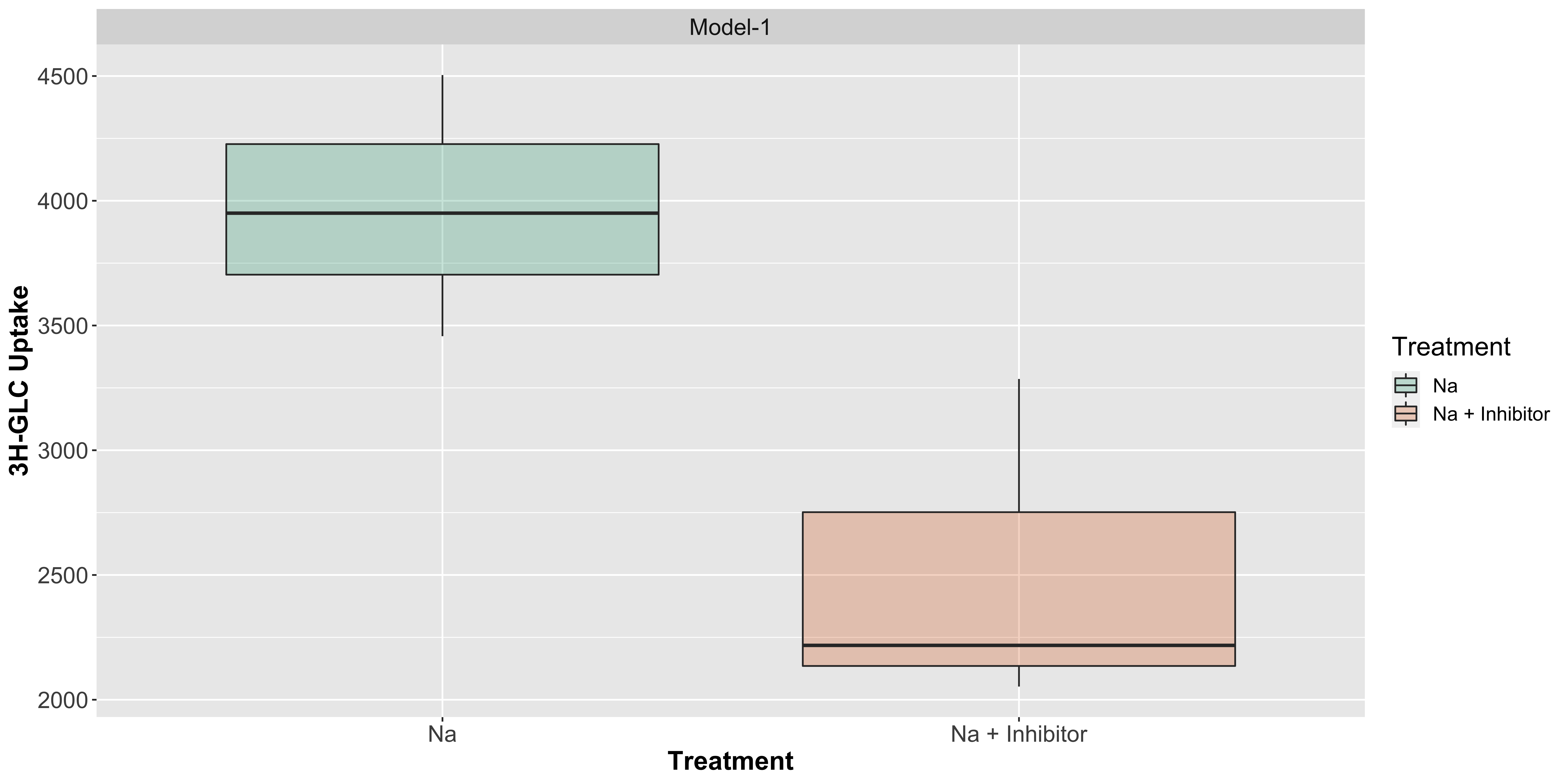 Let us visualize it through a boxplot with points:
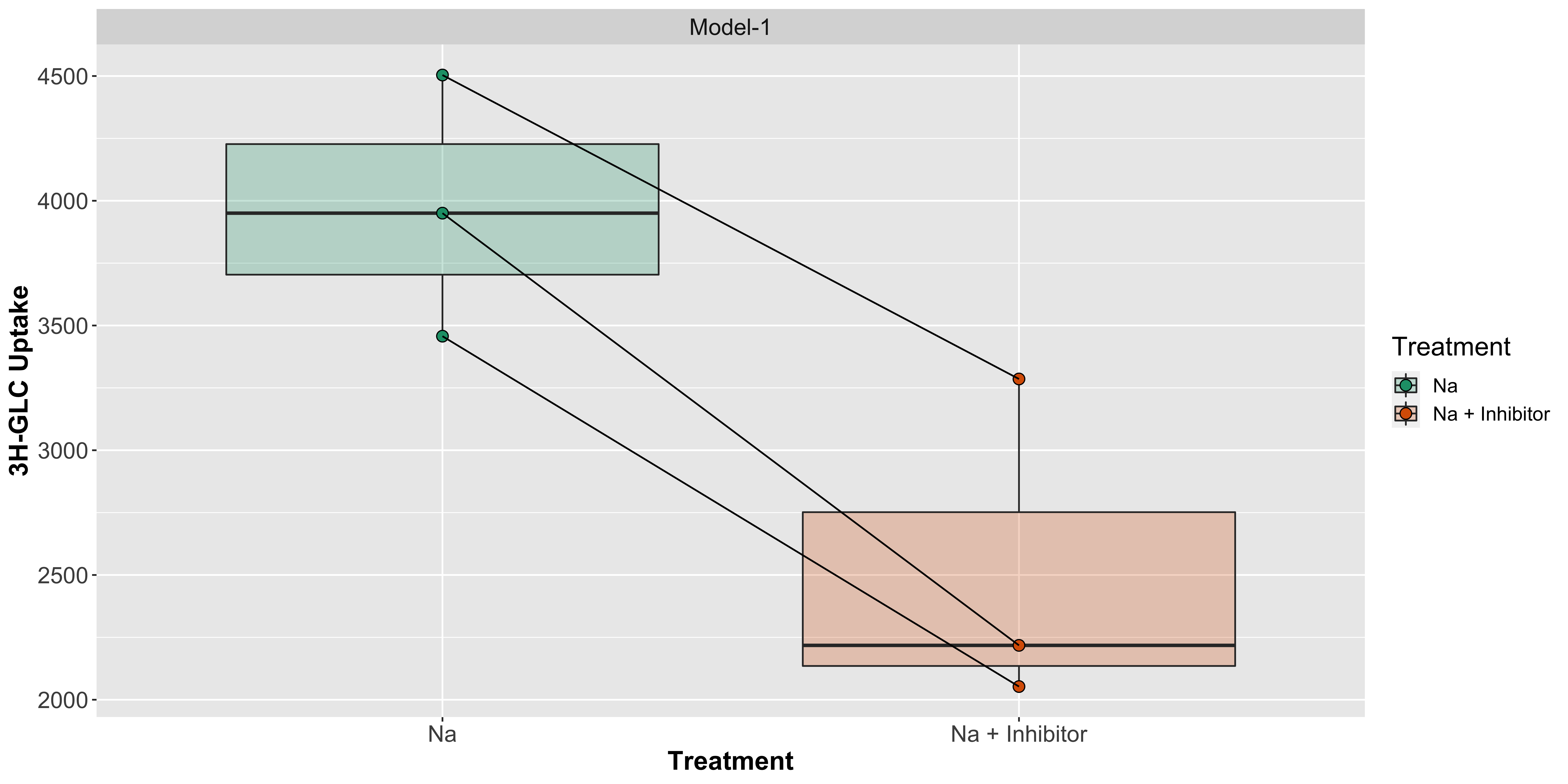
	print(baseplot + boxp + pointPlot) +
	  theme(axis.text=element_text(size=14),axis.title=element_text(size=16,face="bold"),strip.text.x = element_text(
	    size = 14),legend.title = element_text(size=16),legend.text = element_text(size=12))
 Let us visualize it through a boxplot with points and now with the pairing by using lines:
	print(baseplot + boxp + pointPlot + linePlot) +
	  theme(axis.text=element_text(size=14),axis.title=element_text(size=16,face="bold"),strip.text.x = element_text(
	    size = 14),legend.title = element_text(size=16),legend.text = element_text(size=12))
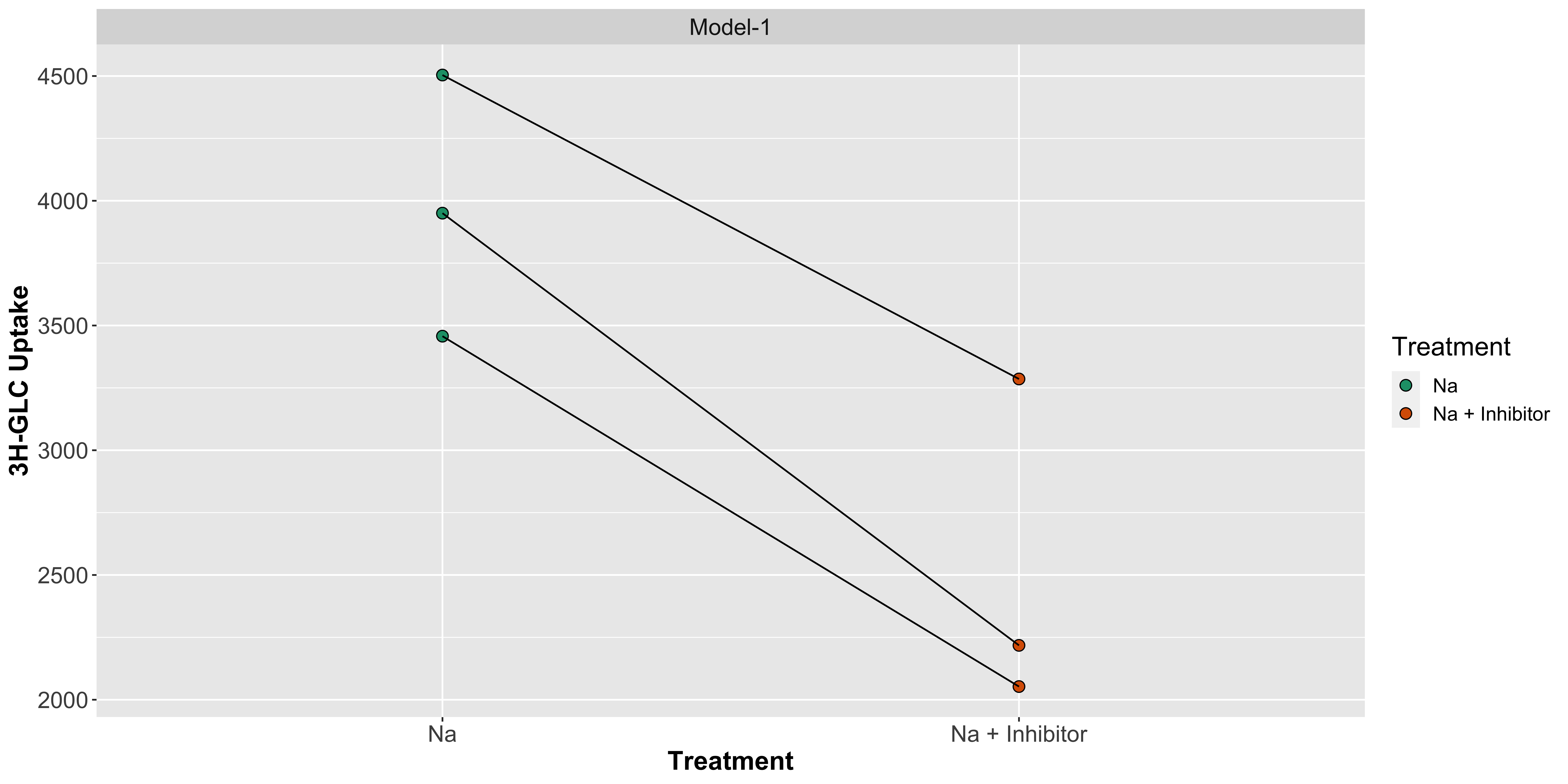
 We can also visualize it without the box but showing the pairing by using lines:
	print(baseplot + pointPlot + linePlot) +
	  theme(axis.text=element_text(size=14),axis.title=element_text(size=16,face="bold"),strip.text.x = element_text(
	    size = 14),legend.title = element_text(size=16),legend.text = element_text(size=12))
 Now, let us run the paired t-test.
t.test(Uptake ~ Treatment, paired=T, data=uptake)
		Paired t-test

	data:  Uptake by Treatment
	t = 9.6597, df = 2, p-value = 0.01055
	alternative hypothesis: true difference in means is not equal to 0
	95 percent confidence interval:
	  805.0936 2098.3617
	sample estimates:
	mean of the differences
				   1451.728
References
Devore, J.L. (2010). Probability and Statistics for Engineering and the Sciences (Eighth ed). Cengage Learning, Boston, MA, USA. https://faculty.ksu.edu.sa/sites/default/files/probability_and_statistics_for_engineering_and_the_sciences.pdf
Motulsky, H. (2018). Intuitive biostatistics : a nonmathematical guide to statistical thinking (Fourth edition. ed.). New York: Oxford University Press. pp. 318-328.
Elston, R.C. and Johnson, W.D. (2008). Basic Biostatistics for Geneticists and Epidemiologists: A Practical Approach. John Wiley & Sons Ltd, West Sussex, UK.