BMR 617: Statistical Techniques for the Biomedical Sciences

Hypothesis Testing

Statistical hypothesis testing is Assessing evidence provided by the data in favor of or against some claim about the population.

Using our usual mouse metabolic data set, let’s just look at body weight of the two groups of mice fed the standard Chow diet

library(tidyverse)
met <- read_csv("https://denvirlab.marshall.edu/BMR617-2022/data/TH-B6-metabolic.csv")
met <- separate(met, MouseID, sep="-", into=c("Strain", "Diet", "ID"))
chow_only <- filter(met, Diet=="Chow")
ggplot(chow_only, aes(x=Strain, y=BodyWeight)) + geom_boxplot() +  geom_point()
	

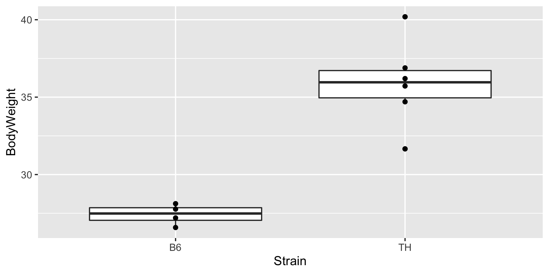
In this example, we are going to test the hypothesis that the strain affects body weight, i.e. that the body weight is different in different strains

The Null Hypothesis

Hypothesis testing is always formulated as testing two competing hypotheses. Generally speaking:

• The null hypothesis is the “default”; i.e. the hypothesis we would tend to conservatively believe without any evidence to the contrary
• The alternative hypothesis is (typically) the hypothesis we want to prove

The null and alternative hypotheses should be mutually exclusive and exhaustive (i.e. one and only one of them is true)

Hypothesis Testing Example

The Null Hypothesis is Always Possible (no matter the data)

Note that our data (and no data) cannot prove beyond any doubt that the alternative hypothesis is true.

The hypothesis concerns the entire population (all possible TH and B6 mice). We only have data from a small sample Since the data vary, even if the null hypothesis is true, there is always some chance that we just happened to sample one group of data predominantly from one side of the distribution, and one group of data from the other.

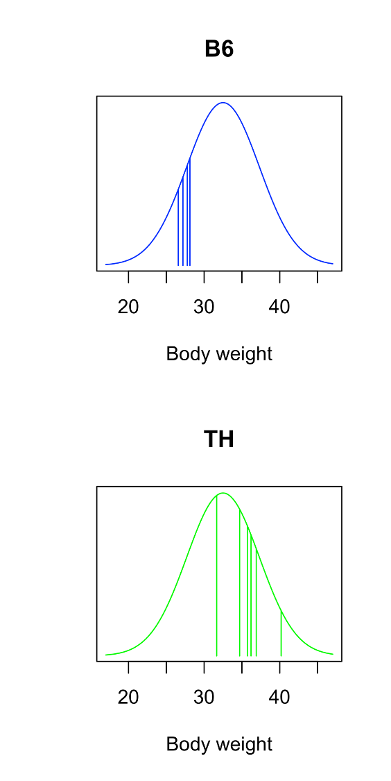
The graphs illustrate the null hypothesis, with the mean (population) body weight of both strains around 32.5g In this scenario, it just happened that our B6 samples came from the left of the distribution, and our TH samples came from the right of the distribution Essentially, we are interested in how likely this scenario is (or isn’t) Unfortunately, we can’t actually measure or calculate this!

Aside: Mathematical Proof

In math, we prove things with complete certainty. For example, it is true that no rational number (i.e. no fraction) is equal to the square root of 2. To prove this, we cannot possibly test all fractions. So our strategy is to assume the statement is false, and show this leads to a contradiction This is called a “proof by contradiction” (it is not the only way of proving something mathematically, but it's a useful and common technique).

Show the proof

Hypothesis Testing: Process

In statistical hypothesis testing, we cannot prove anything completely. Since the data are subject to randomness, we can only talk about probabilities. The approach is similar to a “proof” by contradiction:

• We collect data to provide evidence for our hypothesis of interest (the alternative hypothesis)
• We then assume that the null hypothesis is true (i.e. that the hypothesis of interest is false)
• Under this assumption, we calculate how likely it is we would observe data at least as “extreme” as the data we actually observed.
• If this probability is small, we reject the null hypothesis and conclude that the alternative hypothesis is true.

The p-value

In hypothesis testing, we calculate the probability that, assuming the null hypothesis is true, we would obtain data at least as extreme as the data we observe.

For example, in the B6 vs TH body weights, under the Chow diet, the mean body weight for B6 mice is 27.4g and for TH mice is 35.9g. The difference is 8.5g.

So when we calculate the p-value, we are asking the question: “If the body weights of B6 and TH mice came from distributions with the same mean, what is the probability we would see a difference of at least 8.5g in our samples?”

Calculating p-values

The basic idea is to find a test statistic which takes on a particular value when the null hypothesis is true. We want a test statistic for which the distribution is known when the null hypothesis is true, usually under some additional assumptions. We can then calculate the probability of obtaining data which gives us a test statistic at least as extreme as the one we actually observed.

The combination of a test statistic, and its distribution when the null hypothesis is true, is called a hypothesis test. Much of the remainder of the course will be concerned with learning about different hypothesis tests.

Example: the t-test

If we make the assumption that the body weights of Tallyho and B6 mice are normally distributed, then the quantity \[t = \frac{m_{\operatorname{TH}} - m_{\operatorname{B6}}} {\sqrt{\frac{s_{\operatorname{TH}}^2+s_{\operatorname{B6}}^2}{2n}}}\] is distributed according to a t-distribution with a number of degrees of freedom depending on \(n\). Here \(m_{\operatorname{TH}}\) and \(m_{\operatorname{B6}}\) are the sample means for the TH mice and B6 mice, respectively; \(s_{\operatorname{TH}}\) and \(s_{\operatorname{B6}}\) are the sample standard deviations for the TH mice and B6 mice, respectively, and \(n\) is the number of mice in each sample. There are variations of this if the sample sizes are not equal: more details will be a little later in the course.

t-test in R

R has a t.test function for performing t-tests. Try the following:

library(tidyverse)
met <- read_csv("https://denvirlab.marshall.edu/BMR617-2022/data/TH-B6-metabolic.csv")
met <- separate(met, MouseID, sep="-", into=c("Strain", "Diet", "ID"))
chow_only <- filter(met, Diet=="Chow")
t.test(BodyWeight ~ Strain, data=chow_only)
	

The R syntax BodyWeight ~ Strain is an R formula. This is not a mathematical formula; it expresses the idea that BodyWeight is the response variable, and Strain is an explanatory variable. Again, we will see this in more detail later in the course.

The output from the t-test above is

	Welch Two Sample t-test

data:  BodyWeight by Strain
t = -7.1346, df = 5.8412, p-value = 0.0004303
alternative hypothesis: true difference in means is not equal to 0
95 percent confidence interval:
 -11.402024  -5.549642
sample estimates:
mean in group B6 mean in group TH 
        27.41750         35.89333 
    

The p-value is 0.0004303, or 0.04303%. The interpretation of this is Since this p-value is small, i.e. the chances of getting data like this are highly unlikely if the null hypothesis is true, we would typically reject the null hypothesis and conclude that TH mice have different body weights to B6 mice when fed a chow diet.

Interpreting Hypothesis Tests

Care is needed in interpreting a hypothesis test.

These are very commonly misinterpreted, even by advanced professional scientists.

In our test, the p-value was 0.00043 So, if there were no difference in body weight between B6 and TH mice, there would be only a 0.043% chance of obtaining a difference in means this big with these sample sizes. Since this is so unlikely, we would reject the null hypothesis and conclude that the two strains had different body weights.

As we'll see, this is not the same as saying "the probability the null hypothesis is true is 0.00043".

We must also be careful not to over-interpret "large" p-values.

p-value thresholds

The natural question here is “how small is a small p-value?”

The standard approach is to choose a threshold, below which we will reject the null hypothesis. We do this before collecting and analyzing data.

Hypothesis testing was invented in the late 1800s by Ronald Fisher. In his original paper, as an example, he used a threshold of 0.05 This has become, for no particularly good reason, a “standard” threshold

Important lesson #1: The p-value is not the probability the null hypothesis is true

The p-value is the probability of obtaining data as extreme as that observed, under the assumption that the null hypothesis holds.

This is not the same as the probability that the null hypothesis is true, though it is commonly mistaken as such.

We can almost never compute the probability the null hypothesis is true.

Illustrative scenario

Prof. Cavendish O’Leary (“Cav”) runs a lab in the Institute for Unlikely Discoveries. Over the course of his career, he conducts 1000 studies. His ambition is to discover something that will make him famous and chooses studies that, if successful, will be groundbreaking and paradigm shifting in the field.

Prof. Prudence Dent (“Pru”) runs a lab in the Institute for the Establishment of Known Facts. Over the course of her career, she also conducts 1000 studies. Her aim in life is to build a steady body of solid, reproducible publications, and as such she only studies things with an abundance of solid evidence.

The a-priori probability

Because Cav O’Leary and Pru Dent exist only in a fictional universe, of which we are the creators and omnipotent beings, we know that 2% of the hypotheses that Prof. O’Leary tests are really true, and that 90% of the hypotheses that Prof. Dent tests are really true.

These values are called the a-priori” probabilities of the hypotheses, and these are never known in the real world.

Both Prof. O’Leary and Prof. Dent use a p-value threshold of 0.05 to determine "statistical significance" (i.e. to decide whether or not to reject the null hypothesis).

Furthermore, both design their experiments and choose their sample sizes to give a statistical power of 80%: if their hypothesis is true, there is an 80% chance they will get a p-value less than the threshold.

The question we want to ask is: if Prof. Pru Dent performs an experiment and gets a "significant" p-value (i.e. \(p < 0.05\)), what is the probability her hypothesis is true (and the null hypothesis is false)? What about the same question for Prof. O'Leary?

1000 Experiments with an a-priori probability of 90%

		Reject Null Hypothesis
		No	Yes	Total
Null hypothesis really true	Yes
	No
	Total			1000

1000 Experiments with an a-priori probability of 2%

		Reject Null Hypothesis
		No	Yes	Total
Null hypothesis really true	Yes
	No
	Total			1000

Conclusions

Many people assume that if we reject the null hypothesis (with a p-value threshold of 0.05), it means there is a 95% chance the null hypothesis is false (i.e. that the hypothesis of interest is true).

This fictional scenario demonstrates this is not true.

The probability the null hypothesis is false, given we have a p-value less than 0.05, depends greatly on the a-priori probability.

• The prior probability that the null hypothesis was false.

The problem is, again, that we never actually know this. In our (somewhat extreme) examples, the probabilities we calculated were 0.993, and 0.246,respectively.

Important lesson #2: A "non-significant" p-value doesn’t lead to any conclusion

In the hypothesis-testing scenario, we choose a p-value threshold (below which we reject the null hypothesis).

We then collect data and perform our analysis, computing the p-value.

If the p-value is below the threshold, we reject the null hypothesis and conclude the hypothesis of interest is correct.

If the p-value is above the threshold, we simply fail to reject the null hypothesis.

• Notice here that we don’t draw any conclusion.
• We certainly cannot conclude the null hypothesis is true.

p > 0.05 is often misinterpreted

This last point is very commonly misunderstood.

It is very common to see statements, even in published papers, like "There was no difference in the blood pressures of patients on drug A or drug B (\(p>0.05\))"

• This is not a valid conclusion from a “non-small” p-value!
• At best, you can conclude that the experiment or study failed to demonstrate a difference.

Further Reading

In March 2019, the American Statistical Association published a special edition of their journal, The American Statistician, addressing misunderstandings of hypothesis testing and p-values.

Read (as a minimum) the editorial from this issue.

Nature published an accompanying article, signed by 800 academic and professional statisticians.

The key point these articles make is to stop categorizing and dichotomizing results based solely on p-values. Instead, thoughtfully assess all the data and analyses.