BMR 617: Statistical Techniques for the Biomedical Sciences

Confidence Intervals

Last time:

We looked at the Cholesterol levels for our sample of six TH mice fed Chow. We calculated the mean of the sample, and a 95% confidence interval of the mean.

The mean was 101.2 mg/dl, with a 95% confidence interval \([93.2, 109.2]\).

The interpretation of this is that we are 95% confident that the interval (range) \([93.2, 109.2]\) contains the true mean Cholesterol level for Tallyho mice fed a Chow diet.

Understanding Confidence Intervals

Let's dissect that interpretation a little.

• The "true mean Cholesterol level" (\(\mu\)) is a fixed, unknown quantity.
  • If we were to repeat the experiment, the "true mean Cholesterol level" doesn't change (and still remains unknown)
• The sample mean (\(m\)) is computed from our data. It is our estimate of the true value \(\mu\). If we repeat the experiment multiple times, we'll get a different value for \(m\) each time.
• The confidence interval \([93.2, 109.2]\) represents a range of values. For estimates of the mean, assuming the data are sampled from a normal distribution, the interval will be centered at the sample mean. If we repeat the experiment many times, we'll get a different interval each time
• The "95%" is a value we chose, and is called the "level of confidence". Note that we chose to compute a 95% confidence interval (which is traditional). We could just have easily have chosen a 90% confidence interval, or a 99% confidence interval, etc.

Random Variables

In statistical language, we say that the sample mean is a Random Variable, because its value depends on random effects. If we measure it multiple times, we'll get different values each time.

The confidence interval is also a random variable, because we get different confidence intervals for each data set we sample.

The population mean, which we don't know, is not a random variable, because its value is fixed.

Note that we've always used the language

We are 95% confident the interval \([93.2, 109.2]\) contains the true Cholesterol value for TH mice fed a Chow diet.

It's tempting to say

We are 95% confident the true Cholesterol value lies in the range \([93.2, 109.2]\).

While this is logically true, it feels slightly misleading, because it implies the "true mean" can vary.

Simulating Confidence Intervals

To get a feel for confidence intervals, we'll run a simulation. The idea here is to simulate a large number (say 100) of experiments similar to the one in which we measured the cholesterol levels of six TH mice fed a Chow diet.

We're going to need to be able to compute margins of error for a set of values, assuming they're sampled from a normal distribution. In order to make this easy in R, we can define a function to do this. We want this function to take a set of values and a confidence level, which will have a default value of \(0.95\).

The code to do this is

	
marginError <- function(x, confidenceLevel = 0.95) {
  n <- length(x)
  sem <- sd(x) / sqrt(n)
  p <- (1 + confidenceLevel) / 2
  critT <- qt(p, df = n - 1)
  marginError <- critT * sem
  marginError
}
	
	

First, let's check this does what we expect. Then we'll examine this code line-by-line.

The cholesterol values for these six mice are

• 107.98
• 97.55
• 89.57
• 99.23
• 102.31
• 110.77

The margin of error we calculated last time was 8.01. Try

	
	marginError(c(107.98, 97.55, 89.57, 99.23, 102.31, 110.77))
	
	

and make sure you get what you expect.

The code

	marginError <- function(...) { 
	  ...
	}
	
	

defines a function which we name marginError. When we call this function, the commands between the { ... } are executed. The last value evaluated is the value of the function.

There are two parameters in this function, x and confidenceLevel. These are values (data) passed to the function. x is the set of values for which we compute the margin of error. confidenceLevel is the confidence level we need. The confidenceLevel = 0.95 in the function definition provides a default value for confidenceLevel. This means if we don't provide a value, it will be assumed to be 0.95.

The rest of the function just calculates the margin of error, essentially as we did before. The only tricky part here is the value to pass to qt. Remember that for a 95% confidence level, we figured that 1-0.95 lay outside the central area in the t-distribution, and then we divided that by two to get the region to the right of the region of interest, giving \[\frac{1-0.95}{2}=0.025\] The value we needed was the area to the left of this, so we then subtracted that from 1: \[1 - \frac{1-0.95}{2} = 0.975\] In general, for a confidence level \(c\), we need \[1 - \frac{1-c}{2} = 1 - \left(\frac{1}{2}-\frac{c}{2}\right)=1-\frac12+\frac{c}2=\frac12+\frac{c}2=\frac{1+c}{2}\] So in code we do

	p = (1 + confidenceLevel)/2
	

and then

	critT = qt(p, df = n-1)
	

To recap, the whole function looks like

marginError <- function(x, confidenceLevel = 0.95) {
  n <- length(x)
  sem <- sd(x) / sqrt(n)
  p <- (1 + confidenceLevel) / 2
  critT <- qt(p, df = n - 1)
  marginError <- critT * sem
  marginError
}
	

To do the actual simulation, we need some values. We're going to generate 6 values for each simulated experiment, and we want 100 experiments. So we need 600 values from a normal distribution. We'll make these look similar to our real data with a mean of 101.2 and a standard deviation of 7.63.

Don't run this yet, but we'll need

Cholesterol = rnorm(600, mean=101.2, sd=7.63)
	

We'll also need to keep track of which simulated experiment each data point belongs to, so we'll create a table with one column representing the Cholesterol value, and the other representing the simulation:

simulChol <- tibble(
  Cholesterol = rnorm(600, mean=101.2, sd=7.63),
  Simulation = rep(1:100, each=6) 
)
	

Have a look at what this looks like (note each time you run this, you'll get different values):

simulChol
	

Now we'll get a confidence interval for each of the 100 simulations. To do this, we'll group the data by each simulation, and for each group calculate the mean, the margin of error, and the upper and lower ends of the confidence interval. We'll also check if the confidence interval contains the "true mean".

simulCholIntervals <- simulChol %>% 
  group_by(Simulation) %>% 
  summarise(
    MeanChol = mean(Cholesterol), 
    MarginError = marginError(Cholesterol, confidenceLevel = 0.95), 
    CILower = MeanChol-MarginError, 
    CIUpper = MeanChol+MarginError, 
    ContainsTrueMean = (CILower<=101.2 & CIUpper>=101.2)
  )
	

Have a look at what this gives you by clicking on simulCholIntervals in the "Environment" tab.

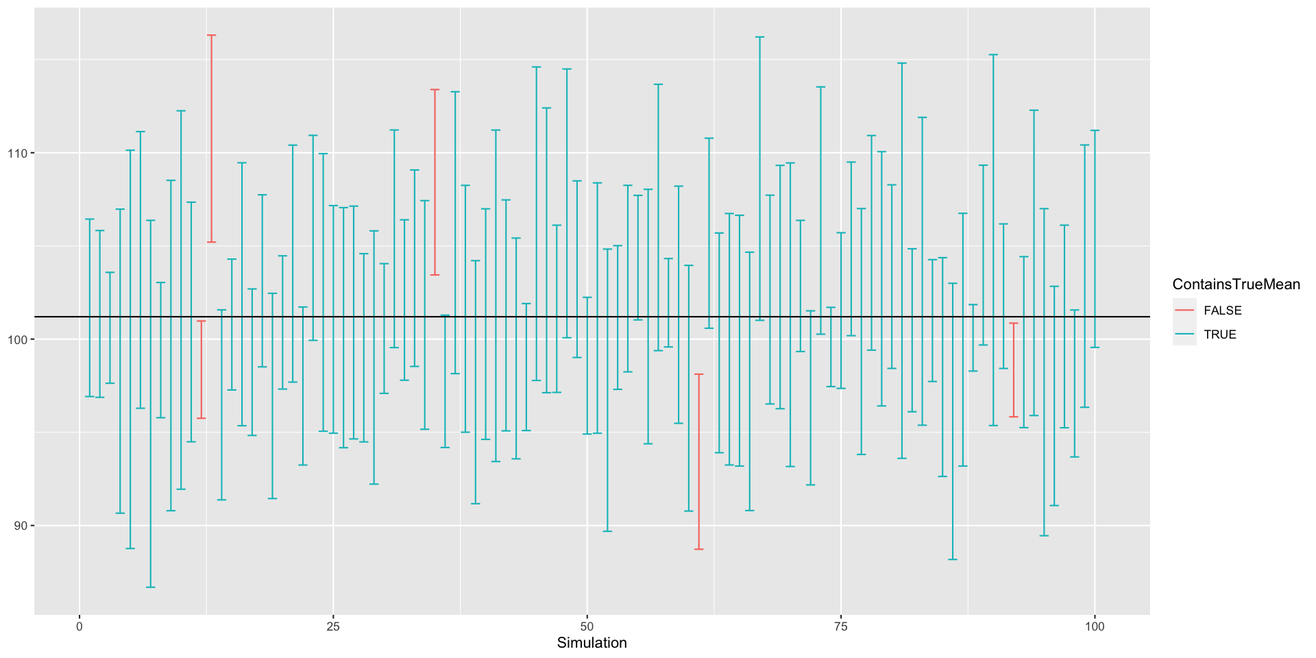
We can also visualize these. Error bars make a nice way to visualize intervals, even without a bar chart:

	
ggplot(simulCholIntervals, aes(x=Simulation, ymin=CILower, ymax=CIUpper, colour=ContainsTrueMean)) + 
    geom_errorbar() + geom_hline(yintercept=101.2)
	
	

How many intervals contain the true mean? How many would you expect on average?

Run the whole simulation again, starting from

simulChol <- tibble(
  Cholesterol = rnorm(600, mean=101.2, sd=7.63),
  Simulation = rep(1:100, each=6) 
)
	

How many intervals contain the true mean this time? Repeat this a few times.

Experiment with running the simulation with different confidence levels.

(Advanced) Write a function that performs the simulation. The parameters for the function should include a confidence level, and might also include the sample size (we used 6), the number of simulations (we used 100), the mean, and the standard deviation of the data.