BMR 617: Statistical Techniques for the Biomedical Sciences
Samples and Populations
Remember the framework we set up last time:
In statistics, we work with data from a sample. Typically, we want to use those data to make inferences about the distribution of values in a population.
For quantitative data, we can compute the mean of the values in our sample. The sample mean provides the best estimate, given our sample data, of the population mean. As well as estimating the population mean, we want to get some information about how close our estimate is likely to be to the true population mean.
So, for example, in our mouse metabolic data, we measured the mean cholesterol level for our sample of six Tallyho mice fed a Chow diet to be 101.2 mg/dl. This is our best estimate for the "true" mean Cholesterol level for TH mice fed a Chow diet, but we'd also like to know how close it is like.ly to be to the true value.
The general way we measure this precision is to try to understand what the distribution of all sample means looks like. To make this a little more concrete, imagine repeating our mouse metabolic experiment. We could get another sample of six TH mice, raise them on a Chow diet, and measure their Cholesterol levels after 16 weeks. If we took the mean of those 6 values, we'd get a slightly different mean to the first time we did the experiment. If we repeated the experiment indefinitely, with a new set of six mice each time, we'd get a whole distribution of sample means. Understanding what this distribution looks like provides information about how accurate our sample mean is, considering it as an estimate of the "true" mean.
The Central Limit Theorem gives us some information about this:
The means of a sample of size \(n\) drawn from a population with mean \(\mu\) and standard deviation \(\sigma\) are approximately normally distributed, with mean \(\mu\) and standard deviation \(\frac{\sigma}{\sqrt{n}}\).
Let's emphasize some points about this:
- It doesn't matter what the actual distribution of the underlying population is. It doesn't need to be normally distributed; it could be highly skewed, multi-modal, etc. The distribution of the sample means will still be approximately normal.
- The distribution of the sample means is not exactly normally distributed; it is only an approximation. This approximation improves as \(n\) gets bigger. So for small sample sizes it might be noticeably non-normal. In practice, if \(n\geq15\) or so, the approximation is very good.
- The standard deviation of the sample means, \(\frac{\sigma}{\sqrt{n}}\) relies on the standard deviation of the population, \(\sigma\), which we typically don't know.
Today we'll look at some refinements of this approach, and deal with the two issues in the last two bullet points, in certain circumstances. First note that we can write the central limit theorem slightly differently: \[\frac{m}{\frac{\sigma}{\sqrt{n}}}\] is approximately normally distributed with mean \(\mu\) and standard deviation \(1\), where \(m\) is the sample mean, \(\mu\) is the population mean, and \(\sigma\) is the population standard deviation. Equivalently, we can say that \[\frac{\mu-m}{\frac{\sigma}{\sqrt{n}}}\] is normally distributed with mean \(0\) and standard deviation \(1\).
One problem we noted last time was that we don't know \(\sigma\). We only know \(s\), the sample standard deviation. So we cannot compute \(\frac{m}{\frac{\sigma}{\sqrt{n}}}\), we can only compute \[\frac{m}{\frac{s}{\sqrt{n}}}\] This is still approximately normally distributed, but this approximation may actually be fairly poor, particularly for small samples size \(n\).
The t-distribution
In the 1920s, the statistician William Sealy Gosset calculated what the actual distribution of \[\frac{\mu-m}{\frac{s}{\sqrt{n}}}\] was, under the additional assumption that the samples are drawn from a normal distribution.
He called this distribution (which is actually a family of distributions) the t-distribution with \(n-1\) degrees of freedom. Like the normal distribution, there are tables, or software, that give values of this distribution.
When the sample size \(n\) is large, the t-distribution closely resembles the normal
distribution. However for small values of \(n\) it looks quite different.
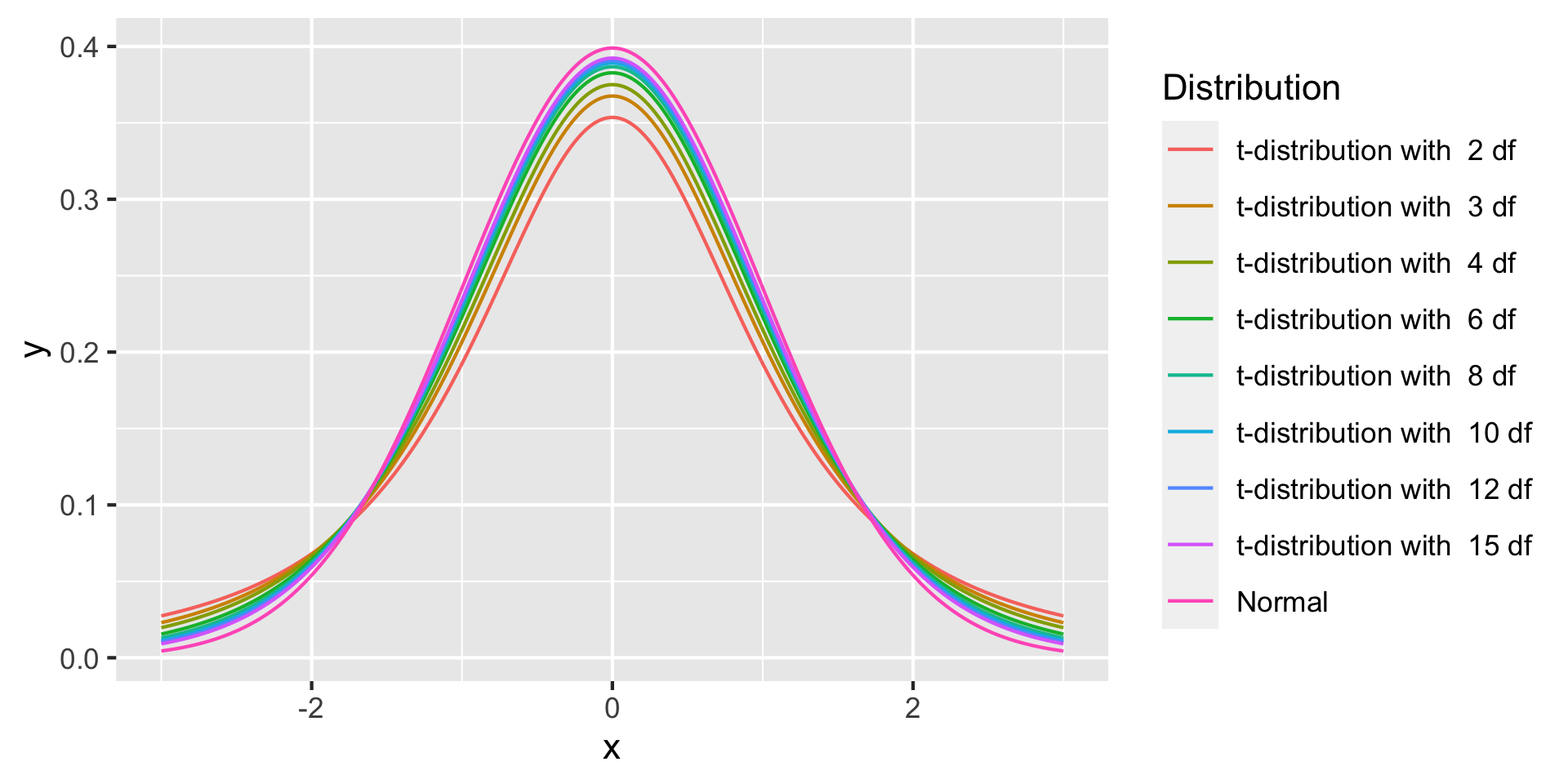 In particular, note that for small degrees of freedom (i.e. small sample sizes \(n\)),
the "tails" of the distribution are much larger. We noted before that for the
normal distribution, about 5% of values were more than 2 standard deviations
from the mean. For the t-distribution, particularly with a small number of degrees
of freedom, this value is much larger.
In particular, note that for small degrees of freedom (i.e. small sample sizes \(n\)),
the "tails" of the distribution are much larger. We noted before that for the
normal distribution, about 5% of values were more than 2 standard deviations
from the mean. For the t-distribution, particularly with a small number of degrees
of freedom, this value is much larger.
Confidence intervals and the t-distribution
Let's apply these ideas to our TH Chow mice cholesterol data, and then we'll make those ideas more general.
Load the data in R, and compute the summary table like we did before:
	library(tidyverse)

	met <- read_csv("https://denvirlab.marshall.edu/BMR617-2021/data/TH-B6-metabolic.csv") %>%
	  separate(MouseID, sep="-", into=c("Strain","Diet","Id"))

	met_summary <- met %>% group_by(Strain, Diet) %>%
	  summarise(Chol=mean(Cholesterol), CholSD = sd(Cholesterol), n=n(), sem=CholSD/sqrt(n))
	met_summary
For the TH Chow group, we have a mean Cholesterol level of \(m=101\), standard deviation
of \(s=7.63\), sample size \(n=6\), and standard error of the mean, \(\frac{s}{\sqrt{n}}=3.12\).
We know that, if we were to repeat this experiment over and over, calculating lots of sample means, the quantity \[t=\frac{\mu-m}{\frac{s}{\sqrt{n}}}\] would follow a t-distribution with \(n-1=5\) degrees of freedom.
Just like we did for the normal distribution, we can find values, which we'll call \(\pm t^*\), so that \[P(-t^*\leq X \leq t^*)=0.95\] Just like before, we note that this is a symmetrical distribution. So if 95% of all values lie between \(\pm t^*\), then 2.5% are more than \(t^*\) and 2.5% are less than \(-t^*\). So we can ask R to find \(t^*\) using
qt(0.975, df=5)
This gives \(2.57\). Note this is quite a bit larger than if we'd use the normal distribution,
which would give a value close to 2.
So we can conclude that if we repeated this experiment many times, 95% percent of the time \[-2.57 < \frac{\mu-m}{\frac{s}{\sqrt{n}}} < 2.57 \] We can rewrite this as \[ -2.57\times\frac{s}{\sqrt{n}} < \mu-m < 2.57\times\frac{s}{\sqrt{n}} \] or \[ m - 2.57 \times\frac{s}{\sqrt{n}} < \mu < m + 2.57\times\frac{s}{\sqrt{n}} \] Or, using our terminology "Standard error of the mean (sem)" \[ m - 2.57 \times\operatorname{sem} < \mu < m + 2.57 \times\operatorname{sem} \]
For our TH Chow mice cholesterol data, we have \(m=101\) and \(\operatorname{sem}=3.12\). \(2.57\times3.12=8.02\), \(101-8.02=92.98\), and \(101+8.02=109.02\), so
In general, given a sample of size \(n\), we can calculate the margin of error for a given confidence level by calculating the corresponding critical t-value from the t-distribution with \(n-1\) degrees of freedom, and multiplying it by the standard error of the mean. The confidence interval for the population mean is the sample mean, plus or minus the margin of error.
Exercise
Add a new column to the summary table, which is the critical t-value for 95% confidence
for each group.
Remember the value to pass to the qt function is \(0.975\),
and the number of degrees of freedom is \(n-1\).
Hint: you can add a new column to the table with
met_summary <- met_summary %>% mutate(criticalT = ...)
Add a second new column, representing the margin of error.
Add two additional columns, representing the two ends of the 95% confidence interval.
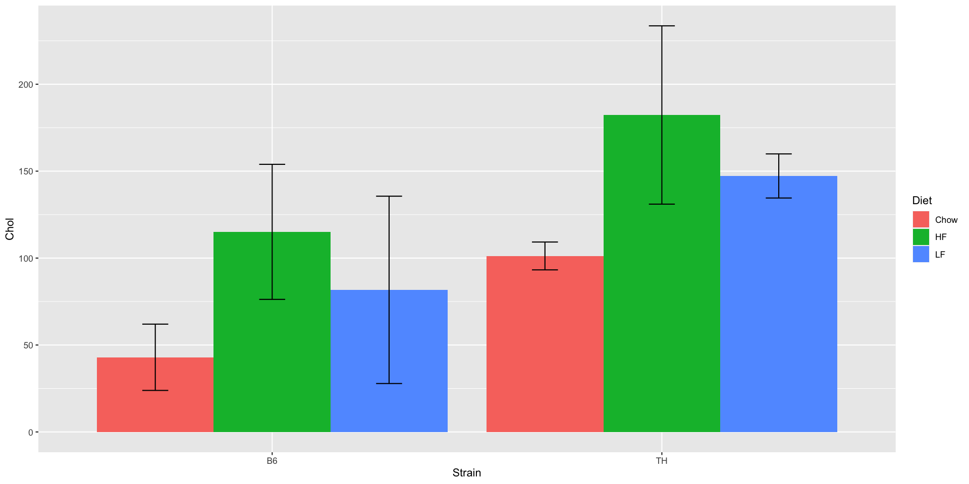
Plot a bar chart, using the 95% confidence interval for the error bars.
You should end up with: