BMR 617: Statistical Techniques for the Biomedical Sciences

Correlation

We previously discussed relative and attributable risks that we used for the C-C case. Today, we will talk about correlation, which is useful for the Q-Q type of relationship.

A correlation exists between two variables when one of the variables is connected/related/associated with the other variable in some way.

If we have enough time, we will also perform some simple commands that you can use within R.

Q-Q Case

You previously saw an example where where the explanatory variable is categorical (Q) and the response variable (outcome) is quantitative, i.e., C-Q case:

Example used was the mouse data, where strain and diet were the categorical explanatory variables and cholesterol levels, triglyceride levels, and fat mass were the quantitative response variables.
Use of boxplots, column scatter plots, and/or bar charts was discussed.
You also estimated the mean, standard deviation, etc.

Last Monday, we saw an example where both explanatory and response variables are categorical, i.e., C-C case:

Example that we used was the BNT162b2 mRNA Covid-19 Vaccine Trial, where treatment and SARS-CoV-2 status were the explanatory and response variables, respectively.
We discussed use of contingency tables, calculation of relative risk, attributable risk, and number needed to treat.

Total, we will consider the type of relationship where both the explanatory and response variables are quantitative, i.e., Q-Q case.

Insulin Sensitivity and Lipid Composition

Borkman et al. (1993) studied the relationship between insulin sensitivity and lipid composition of the cell membrane.

They measured insulin sensitivity of 13 healthy men by infusing insulin and measuring how much glucose they needed to infuse to maintain a constant blood glucose level.

They also took skeletal muscle biopsies and measured (among other things) the percentage of polyunsaturated fatty acids that had between 20 and 22 carbon atoms (%C20-22).

Data

Insulin-Sensitivity Index (mg/m²/min)	%C20-22 Polyunsaturated Fatty Acids
250	17.9
220	18.3
145	18.3
115	18.4
230	18.4
200	20.2
330	20.3
400	21.8
370	21.9
260	22.1
270	23.1
530	24.2
375	24.4

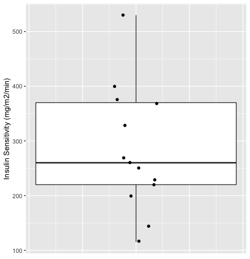
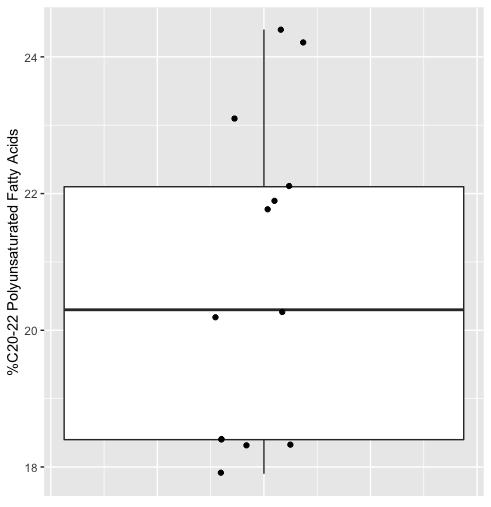
Variability

Both of these variables show a degree of variability

Correlation (or Covariability)

If we plot both variables together in a scatterplot, we see that the variation is "shared" between the variables

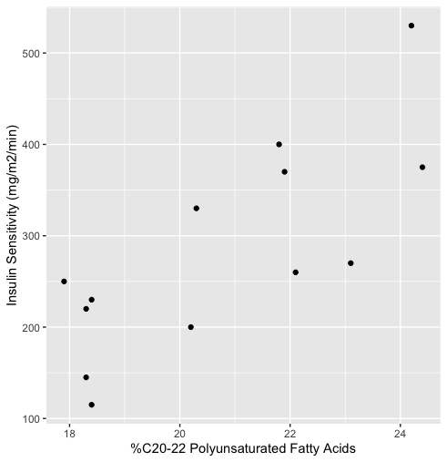
Notice that individuals who have more C20-22 polyunsaturated fatty acids tend to have higher insulin sensitivity.

We say there is a lot of covariability or correlation, i.e., the variables "vary together."

Correlation Coefficient

The amount of correlation can be quantified by a correlation coefficient.

The correlation coefficient between two sets of values x₁..x_n and y₁..y_n is computed as follows:

Calculate the standardized values of x and y: $$ { z_{x,i} = \frac{x_{i} - \bar{x}}{sd(x)} } $$ $$ { z_{y,i} = \frac{y_{i} - \bar{y}}{sd(y)} } $$
Compute the products of all the standardized values, add them up, and divide by n-1: $$ { r = \frac{z_{x,1},z_{y,1} + z_{x,2},z_{y,2} + ... + z_{x,n},z_{y,n}}{n-1} } $$

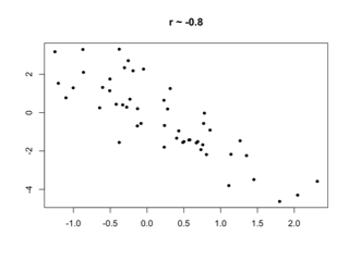
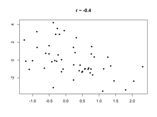
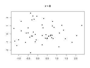
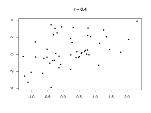
Correlation

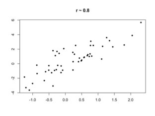
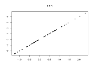
The correlation coefficient between a set of pairs of quantitative values is a measure of the strength of a linear relationship between them.

0 means no linear relationship
1 means a perfect positive linear relationship
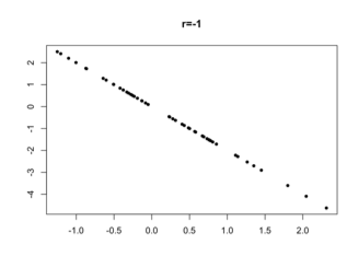
-1 means a perfect negative linear relationship

Why the correlation coefficient works

If a value is bigger than the mean, its standardized score is positive, otherwise its standardized score is negative.

The product of two standardized scores will be positive if both scores are positive, or if both scores are negative, i.e., if both scores are bigger than the mean, or if both are less than the mean.

So if one variable tends to increase when the other tends to increase, the bulk of the products of standardized scores will be positive, and the correlation coefficient will be high.

On the other hand, if one variable tends to decrease when the other increases, the bulk of the products of standardized scores will be negative, and the correlation coefficient will be low.

If there is no relationship, the standardized scores will be randomly distributed, and their products will tend to cancel out.

Computing the correlation coefficient in R

In R, we can do the following:


	cor(pull(ins, `%C20-22`), pull(ins, InsulinSensitivity))

The correlation coefficient for these data is 0.77.

This indicates a strong positive correlation between the two variables.

Interpreting the correlation coefficient

It's usually easier to interpret the square of the correlation coefficient, which we write as 𝑅².

Here R=0.77, so 𝑅²=0.593.

The interpretation of 𝑅² is that it is the proportion of variation that is shared between the two variables, i.e., 59.3% of the variation in insulin sensitivity is associated with the variation in lipid content.

The remaining 40.7% of the variation in insulin sensitivity is explained by other factors.

When dealing with correlation, this is symmetrical, so we can also say that 59.3% of the variation in lipid content is associated with the variation in insulin sensitivity.

Correlation and Causation

There are several possible explanations of the correlation that we observe:

The lipid content of the membranes determines insulin sensitivity.
The insulin sensitivity of the membranes affects its lipid content.
Both lipid content and insulin sensitivity are under the control of another factor.
Lipid content, insulin sensitivity, and several other factors are all part of a complex molecular network.
The two variables do not really correlate, and the observation in this sample was just a coincidence.

We usually say "corelation does not imply causation" -- you might want to read more about this from this page: Correlation vs. Causation

Which explanation is correct?

We'll learn how to quantify (to some degree) the likelihood of the last possibility later.

The only way to decide among the first four options is to do further experiments, where the variables are directly manipulated to see which variable affects which other variable(s).

Caution 1: beware of large samples

Mascaro et al. (2013) published a study where they measured a caregiving score and testes size of 52 fathers of children aged 1-2 years.

They computed a negative correlation between the two variables.

We will discuss the meaning of p<0.05 later in the course.

Note in the figure below that the correlation coefficient R=-0.29.

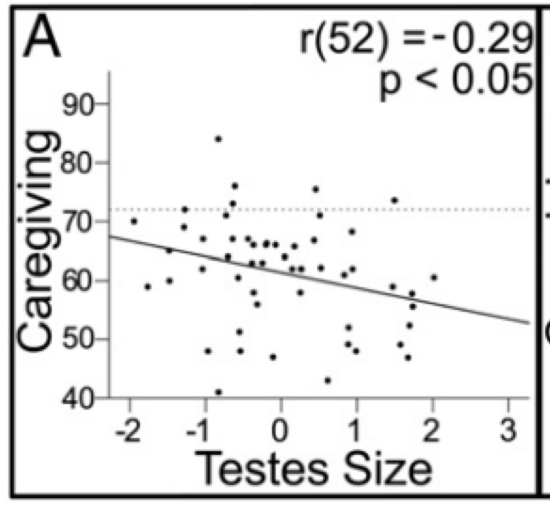
Caption from Fig 1 of Mascaro et al. (2013). "Relationship between reproductive biology and paternal investment. Caregiving vs. testes volume residuals after testes volume was regressed against height. The dotted line indicates the score (72) at which mothers and fathers are equally responsible for their child’s daily care. Scores below 72 imply that the mother does more than the father and scores above 72 imply the opposite."

What is 𝑅²?

0.0823

0.0832

0.0841

0.0855

Incorrect

Try again.

Correct

What is the interpretation?

Diet

91.59% of the variation in paternal caregiving score is associated with the variation in testes size

8.41% of the variation in paternal caregiving score is associated with the variation in testes size

8.41% of the variation in maternal caregiving score is associated with the variation in testes size

Incorrect

In this study, the remaining 91.59% of the variation in paternal caregiving score is explained by other factors.

Incorrect

In this study, the relationship between residual testes volume and paternal caregiving was being tested.

Correct. And remember that when dealing with correlation, the relationship is symmetrical, i.e., 8.41% of the variation in testes size is associated with the variation in paternal caregiving score.

Caution 2: beware of confounding variables

In our mouse data, we could look at correlation between the metabolic variables.

For example, to look at the correlation between Triglycerides and Glucose, we would do:


	met <- read_csv("https://denvirlab.marshall.edu/BMR617-2021/data/TH-B6-metabolic.csv")
	met <- separate(met, MouseID, sep="-", into=c("Strain", "Diet", "ID"))
	cor(pull(met, TG), pull(met, Glucose))

This gives an apparently very strong correlation of 0.878.

A closer look at the Triglycerides-Glucose data

Plot the data:


	ggplot(met, aes(x=TG, y=Glucose)) + geom_point(aes(color=Diet, shape=Strain))

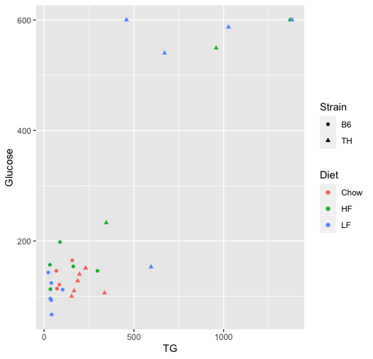
The correlation is "driven" by a few data points which have much higher triglyceride and glucose levels.

Those data points are all TH mice on either the low fat (LF) or high fat (HF) diets.

Within any group, there is little to no evidence of correlation.

So it is likely that Strain and Diet affect both variables, but otherwise the two are unrelated.

References

Borkman, M., Storlien, L. H., Pan, D. A., Jenkins, A. B., Chisholm, D. J., & Campbell, L. V. (1993). The relation between insulin sensitivity and the fatty-acid composition of skeletal-muscle phospholipids. N Engl J Med, 328(4), 238-244. doi:10.1056/NEJM199301283280404.

Motulsky, H. (2018). Intuitive biostatistics : a nonmathematical guide to statistical thinking (Fourth edition. ed.). New York: Oxford University Press. pp. 318-328.

Mascaro, J. S., Hackett, P. D., & Rilling, J. K. (2013). Testicular volume is inversely correlated with nurturing-related brain activity in human fathers. Proc Natl Acad Sci U S A, 110(39), 15746-15751. doi:10.1073/pnas.1305579110.