BMR 617: Statistical Techniques for the Biomedical Sciences
The Normal Distribution
Remember from last time: a statistical distribution is a rule (or function) that describes the probability that a variable takes on its possible values.
BMI Example
In the US, approximately 2% of the adult population is underweight (BMI < 18.5), 34% healthy weight (18.5 < BMI < 25), 34% overweight (25 < BMI < 30), and 30% obese (BMI > 30). We can express the BMI of a randomly selected US adult as a probability distribution: \[ \begin{align*}P(X=\text{Underweight}) &= 0.02 \\ P(X=\text{Healthy}) &= 0.34 \\ P(X=\text{Overweight}) &= 0.34 \\ P(X=\text{Obese}) &= 0.3 \end{align*} \] We can depict this distribution using a bar chart or histogram. Since we have presented the data as categorical here, a bar chart is more suitable: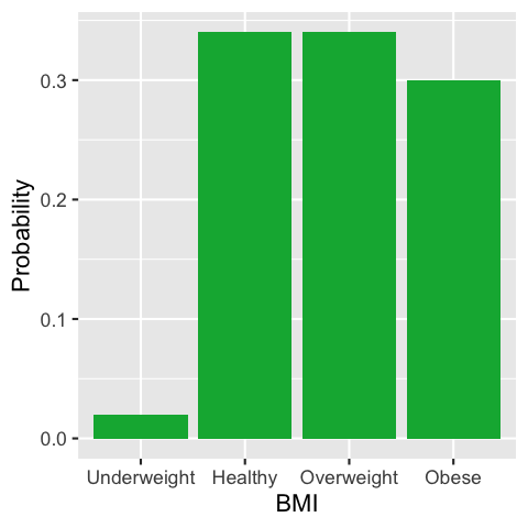 For qualitative variables, in particular those with continuous variables, we cannot talk about the
probability a variable has an exact value; we can only talk about the probability the value lies within
some range.
In this case, the graph of the distribution is interpreted as having an area in any given range equal to the
probability the variable lies in that range.
For qualitative variables, in particular those with continuous variables, we cannot talk about the
probability a variable has an exact value; we can only talk about the probability the value lies within
some range.
In this case, the graph of the distribution is interpreted as having an area in any given range equal to the
probability the variable lies in that range.
We've already seen that the probability the BMI lies in the range 25 to 30 is 0.34 (i.e. 34%), so the distribution
of BMI as a continuous variable might look like:

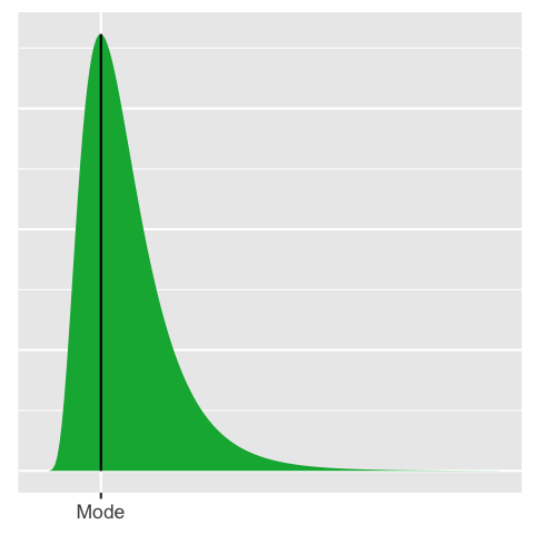
Shapes of distributions
Mode
Symmetry
A distribution is symmetrical if there is some vertical line so that the distribution to the left of the vertical line mirrors the distribution to the right of the vertical line. In a symmetric distribution, the position of the vertical line of symmetry is equal to both the mean and the median of the distribution.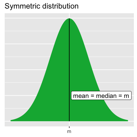
Skewed distributions
A distribution that is not symmetric is called skewed. If the left tail of the graph is longer, then the distribution is called left-tailed, or left skewed, or negatively skewed. If the right tail of the graph is longer, then the distribution is called right-tailed, or right skewed, or positively skewed.
It is a general rule of thumb (though not true for every possible distribution) that in a right-skewed distribution,
the mean is to the right of the median, which in turn is to the right of the mode. Generally, in a left-skewed
distribution, the mean is to the left of the median, which is to the left of the mode.

Examples
- The BMI of all adults in the US is a right-skewed, unimodal distribution.
(It is right-skewed because there are more overweight people than underweight, and
those who are overweight span a wider range of BMIs than those who are underweight.)
Which of the following is most likely?
-
The mean BMI and the median BMI are both equal to 24.
-
The mean BMI is 24 and the median BMI is 25.
-
The mean BMI is 25 and the median BMI is 24.
-
The mean BMI is 21 and the median BMI is 22.
-
The mean BMI and the median BMI are both equal to 22.
Incorrect
In a right-skewed distribution, the mean is typically larger than the median.
Correct!
In a right-skewed distribution, the mean is typically larger than the median.
This answer is the only answer consistent with that.
- What properties would you expect of the distribution of heights of all adult women in the US?
-
Unimodal and highly right-skewed
-
Unimodal and approximately symmetric
-
Unimodal and highly left skewed
-
Bimodal and approximately symmetric
-
Bimodal and highly right-skewed
Incorrect
The mean height of a woman in the USis around 66 inches (5'6).
Women are approximately equally likely to be taller or shorter than this mean,
with values becoming less likely the further you get from the mean.
Correct!
The mean height of a woman in the US is around 66 inches (5'6).
Women are approximately equally likely to be taller or shorter than this mean,
so the distribution is symmetric.
Values becoming less likely the further you get from the mean, so there are no additional
peaks in the distribution.
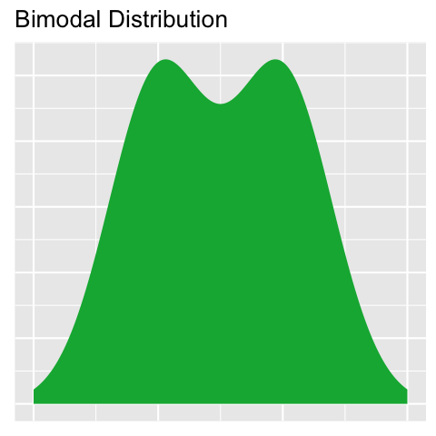
- What properties would you expect of the distribution of heights of all adults (men and women) in the US?
-
Unimodal and highly right-skewed
-
Unimodal and approximately symmetric
-
Unimodal and highly left skewed
-
Bimodal and approximately symmetric
-
Bimodal and highly right-skewed
Incorrect
The mean height of a woman in the US is around 66 inches (5'6),
and the mean height of a man is around 69 inches (5'9).
Both women and men are approximately equally likely to be taller or shorter than the
respective means,
with values becoming less likely the further you get from the mean.
Correct!
The mean height of a woman in the US is around 66 inches (5'6),
and the mean height of a man is around 69 inches (5'9).
Since there are two distinct means, and the number of men and
women are approximately equal, there are likely to be two peaks in the
distribution, so it is likely to be bimodal.
Both women and men are approximately equally likely to be taller or shorter than the
respective means,
with values becoming less likely the further you get from the mean, so
the distribution will be approximately symmetric.
The Normal Distribution
- The mean BMI and the median BMI are both equal to 24.
- The mean BMI is 24 and the median BMI is 25.
- The mean BMI is 25 and the median BMI is 24.
- The mean BMI is 21 and the median BMI is 22.
- The mean BMI and the median BMI are both equal to 22.
- Unimodal and highly right-skewed
- Unimodal and approximately symmetric
- Unimodal and highly left skewed
- Bimodal and approximately symmetric
- Bimodal and highly right-skewed
- Unimodal and highly right-skewed
- Unimodal and approximately symmetric
- Unimodal and highly left skewed
- Bimodal and approximately symmetric
- Bimodal and highly right-skewed
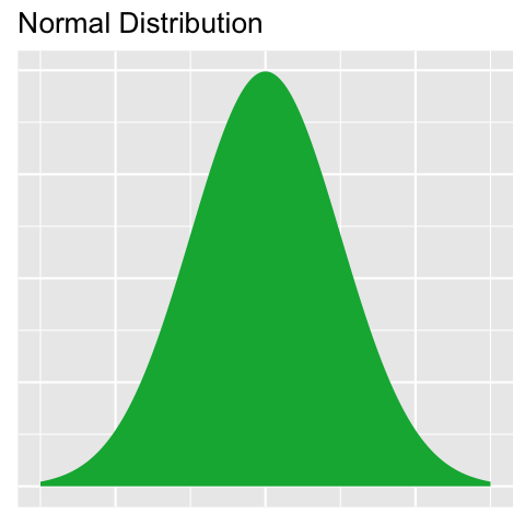
The Normal Distribution is a specific continuous statistical distribution, with several important properties. It was first studied in the 17th century because it had certain theoretical mathematical properties; in the late 19th and early 20th century is was shown that it also occurs widely in nature. This includes occurring frequently in measurements that are routinely taken in clinical and medical science.
The key properties of the normal distribution are:
- It is symmetric
- It is unimodal
- It has a characteristic "bell-shape"
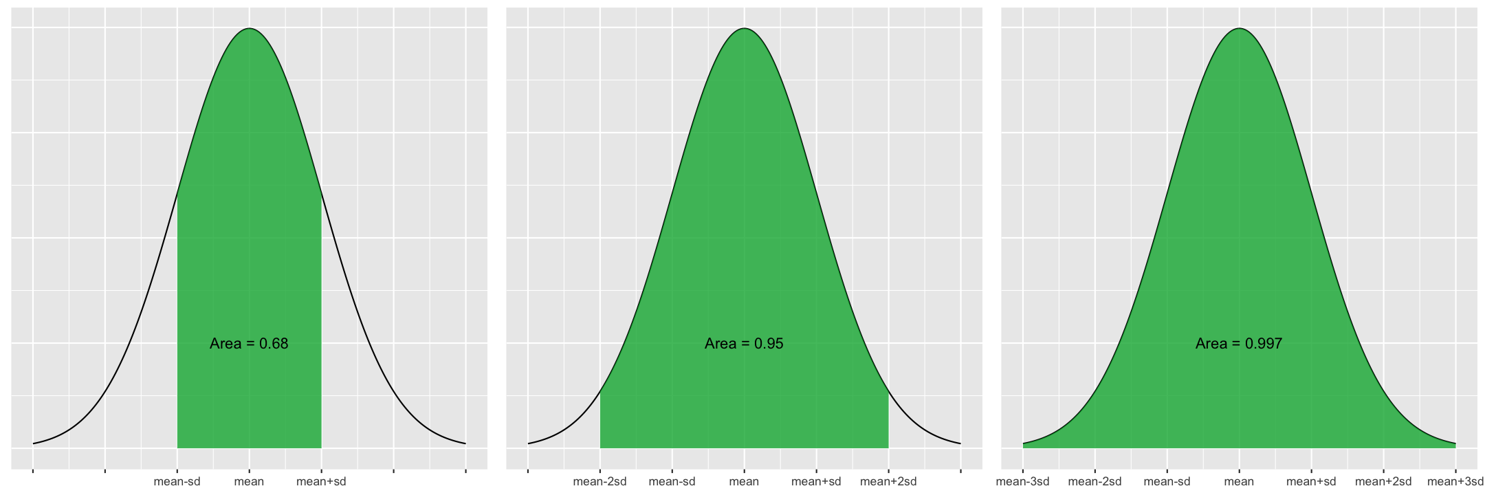
The 68-95-99 rule
In particular, the normal distribution has the property that
- Approximately 68% of all values lie within 1 standard deviation of the mean
- Approximately 95% of all values lie within 2 standard deviations of the mean
- Approximately 99.7% of all values lie within 3 standard deviations of the mean
The standard normal distribution and Z-scores
If \(x\) is a variable sampled from a normal distribution with mean \(\mu\) and standard deviation \(\sigma\), then \(\frac{x-\mu}{\sigma}\) is distributed according to a normal distribution with mean 0 and standard deviation 1.
In other words, subtracting the mean from a normally distributed variable, and then dividing by the standard deviation standardizes the variable. We call the resulting quantity the Z-score for \(x\). The normal distribution with mean 0 and standard deviation 1 is sometimes called the standard normal distribution.
A consequence of this is that if \(x\) is from a normal distribution with mean \(\mu\) and standard deviation \(\sigma\), and \[Z=\frac{x-\mu}{\sigma}\] then
- 68% of the time, \(Z\) will lie between -1 and +1
- 95% of the time, \(Z\) will lie between -2 and +2
- 99.7% of the time, \(Z\) will lie between -3 and +3.
Examples
Assume for these questions that the BMI of males age 60-70 in the US is normally distributed with a mean of 29 and a standard deviation of 6.- What is the Z-score for the BMI of a man in this population with a BMI of 32?
- Z=1
- Z=0.5
- Z=0
- Z=-0.5
- Z=-1
IncorrectRemember, the Z-value is obtained by taking the raw value, subtracting the mean, and dividing the result by the standard deviation.Correct!The Z-value is obtained by taking the raw value, subtracting the mean, and dividing the result by the standard deviation. In this case, \[Z=\frac{32-29}{6}=\frac{3}{6}=0.5\] - Approximately what proportion of men in the US between the age of 60 and 70 have BMI over 35?
- 50%
- 32%
- 16%
- 5%
- 2.5%
IncorrectCompute how many standard deviations this is from the mean, and use the 68-95-99 rule.Correct!35 is 29+6, so it is one standard deviation above the mean.
By the 68-95-99 rule, 68% of men age 60-70 in the US have BMI within one standard deviation of the mean, i.e. between 23 and 35.
Because the normal distribution is symmetric, the remaining 32% are equally split between those with BMI above 35 and those with BMI below 23.
Consequently, half of those 32%, i.e. 16%, have BMI greater than 35.
Incorrect.You have fallen into a common trap with this kind of question. Some pictures will help. (It always helps to draw a picture for these questions.)The BMI of interest, 35, is 6 more than the mean, which is exactly 1 standard deviation more than the mean. The 68-95-99 rule tells us that 68% of all values lie within 1 standard deviation of the mean.
The remaining values, which account for 100%-68%=32%, lie outside this range.
However, these values include values which are more than 1 standard deviation less than the mean, as well as the values we're interested in: the values that are more than one standard deviation greater than the mean.
Because the distribution is symmetric, half of the values falling outside this range are to the right (greater than 35), and half are to the left (less than 23). So 16% of the BMI values for this population are greater than 35.


- Approximately what proportion of men in the US between the age of 60 and 70 have BMI below 17?
- 50%
- 32%
- 16%
- 5%
- 2.5%
IncorrectCompute how many standard deviations this is from the mean, and use the 68-95-99 rule.Correct!17 is 29-12, so it is two standard deviations below the mean.
By the 68-95-99 rule, 95% of men age 60-70 in the US have BMI within two standard deviations of the mean, i.e. between 17 and 41.
Because the normal distribution is symmetric, the remaining 5% are equally split between those with BMI above 41 and those with BMI below 17.
Consequently, half of those 5%, i.e. 2.5%, have BMI less than 17.
The normal distribution and R
R has functions that give values and calculate probabilities associated with the normal distribution.
The pnorm function calculates probabilities. For example, to calculate the probabilty
that a value in the standard normal distribution (i.e. with mean 0 and standard deviation 1)
is less than -2, we could do
pnorm(-2)
For the last question above: the probability a man aged 60-70 in the US has a BMI below 17, assuming the
mean BMI for that group is 29 and the standard deviation is 6, is
pnorm(17, mean=29, sd=6)
Why does this give the same result as the previous call?
To calculate the probability that a value is larger than some fixed value, we can either do
1 - pnorm(35, mean=29, sd=6)
or we can use the lower.tail parameter:
pnorm(35, mean=29, sd=6, lower.tail=FALSE)
We can use rnorm to generate random values that are drawn from a normal distribution.
For example, if we wanted to simulate the BMIs of 100 US men between the ages of 60 and 70, we could do:
bmis <- rnorm(100, mean=29, sd=6)
Check what you get:
bmis
What does this give you?
bmis >= 35
What about
sum(bmis >= 35)
Is this approximately what you would expect?