BMR 617: Statistical Techniques for the Biomedical Sciences
Exploring Distributions
A statistical distribution is a rule (or function) that describes the probability that a variable takes on its possible values.
Simplest possible example
The prevalence of diabetes (type I or type II) in the US is 10.5%. If the variable X is the diabetes status of a randomly selected person in the US, then X has two possible values: "diabetic", and "not diabetic". The probability distribution is simply \[ P(X=\text{diabetic}) = 0.105\] \[ P(X=\text{not diabetic}) = 0.895 \]
BMI Example
In the US, approximately 2% of the adult population is underweight (BMI < 18.5), 34% healthy weight (18.5 < BMI < 25), 34% overweight (25 < BMI < 30), and 30% obese (BMI > 30). We can express the BMI of a randomly selected US adult as a probability distribution: \[ \begin{align*}P(X=\text{Underweight}) &= 0.02 \\ P(X=\text{Healthy}) &= 0.34 \\ P(X=\text{Overweight}) &= 0.34 \\ P(X=\text{Obese}) &= 0.3 \end{align*} \] We can depict this distribution using a bar chart or histogram. Since we have presented the data as categorical here, a bar chart is more suitable: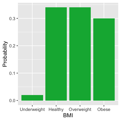
Continuous distributions
In the BMI example above, we made X into a discrete (categorical) variable by breaking it into (essentially arbitrary) ranges. In reality, BMI is a continuous, quantitative variable which can take on any positive value, not necessarily a whole number. In this situation we can no longer talk about the "probability a variable is equal to" some particular number. Why not?
Consider trying to establish if an individual's BMI is equal to 26. BMI is weight (in kilograms) divided by the square of height (in meters). In theory, we could measure both of these quantities to an arbitrary degree of precision. So while an individual might have a BMI of 26 when rounded to the nearest whole number, and maybe even 26.0 when rounded to one decimal place, if we increase the precision enough we will find some difference, no matter how small, between the individual's BMI and the value 26. Consequently, the probability their BMI is exactly equal to 26 is mathematically zero. The same is true for any other value to which we want to compare their BMI!
Instead, we can talk about the probability that an individual's BMI is in some range of values. In this case, the graph of the distribution is interpreted as having an area in any given range equal to the probability the variable lies in that range.
We've already seen that the probability the BMI lies in the range 25 to 30 is 0.34 (i.e. 34%), so the distribution
of BMI as a continuous variable might look like:

Thinking of the probability that the BMI lies in a range, instead of being exactly equal to some number, solves the problem of being equal, given a specific precision. For example, the probability that an individual's BMI is equal to 26 when rounded to the nearest whole number is equivalent to the probability their BMI lies in the range 25.5 < BMI < 26.5. And similarly, the probability it is equal to 26.0 to one decimal place is the probability it lies in the range 25.95 < BMI < 26.05.
Summarizing quantitative data
When working with quantitative data, it's useful to be able to provide some brief summaries of a data set which describe its distribution. Typically we want to know:
- What is a typical or central value of our data?
- How spread out are the data?
Measures of centrality ("Averages")
Computing some kind of average is really a way of finding "the most typical" value in our data set. For quantitative data, there are two averages we typically compute:
- The mean: the sum of all values divided by the number of values
- The median: the "middle" value if they are all placed in order
Loading some sample data
We’ll load a data set that we’ll use frequently throughout this course.
This data set comprises metabolic data from a mouse experiment in Dr. Kim’s lab. Two strains of mouse, C57BL/6 ("B6"") and Tallyho ("TH"") were fed three different diets (standard Chow, the control; a low-fat, high-calorie diet ”LF”, and a high-fat diet “HF”).
Various metabolic measurements were taken from each mouse after 16 weeks on the diet.
We will use the tidyverse library throughout the course to manage our data.
Remember tidyverse is a package (a collection of functions). Packages must
be installed once and once only, with install.pacakges("tidyverse").
We did that last time, so there is no need to do it again (unless you reinstalled R since the last class).
Packages must be loaded once for each R session with the library function:
library(tidyverse)
The data are stored in a comma-separated value (CSV) file.
Once you have loaded tidyverse, you can load the data with the read_csv function:
met <- read_csv("https://denvirlab.marshall.edu/BMR617-2021/data/TH-B6-metabolic.csv")
This will read the CSV file, divide it up into columns at each comma, and rows at each newline,
creating a table. We called the R object holding the table met (of course, you
can call it anything you like). You will now see met in the environment tab:
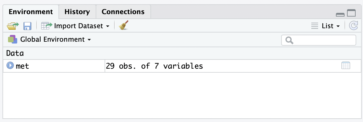
Click on met in the Environment tab to view the data:
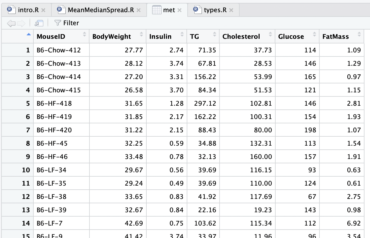
Note that the MouseID column contains the strain (TH or B6), diet (Chow, HF, or LF),
along with a mouse id. We'd like to have access to the strain and diet in a more convenient way.
We can separate that column out into three columns using the tidyverse separate
function. We need to specify what character to use to separate out the new columns (here it is -),
and what the new columns should be called. We do this with:
met <- separate(met, MouseID, sep="-", into=c("Strain", "Diet", "Id"))
Run that command and view the data again.
Mean and Median in R
Let’s focus on just one group of mice. We can do this by filtering the data: (another tidyverse function):
th_chow <- filter(met, Strain=="TH" & Diet=="Chow")
Explain this code
The filter function takes a data table (met in our case)
and a condition. It will create a new data table containing only the rows
in the original table for which the condition is true.
The condition in our case is
Strain=="TH" & Diet=="Chow"
There are two things to explain here. The == (a double equal mark)
is a comparison for equality. It is true if the left hand side is equal to
the right hand side, and false otherwise. Don't confuse this with the single equal
mark =, which means the same as <- (i.e. it assigns a
value to an object.)
The other operator is &, which is "and". It results in a true value
only if the left hand side and the right hand side are both true.
So our filter gets only the rows which have "TH" for Strain and "Chow" for Diet, and
puts them in a new data table which we called th_chow.
Run the code and view the new data table th_chow. Make sure it has only the expected rows.
We can “pull” the cholesterol values from this filtered table:
th_chow_chol <- pull(th_chow, Cholesterol)
Find th_chow_chol in the Environment tab. What data type is this? Is that what you
expected?
To find the mean cholesterol for this group, use
mean(th_chow_chol)
- 100.77
- 101.235
- 102.315
- 102.753
To find the median, use
median(th_chow_chol)
- 100.77
- 101.235
- 102.315
- 102.753
Repeat the previous steps to find the mean and median Cholesterol for the TH HF group.
- 100.77
- 101.235
- 171.17
- 182.31
- 100.77
- 101.235
- 171.17
- 182.31
Mean versus Median
Which measure of central tendency should we use? Mean or median?
- The mean has more useful mathematical properties
- We will discuss these briefly later in the course
- Allows us to do more powerful statistics, such as hypothesis testing
- However, the mean is not ”robust to outliers”
- If one of our values was accidentally recorded with a large error (say by a factor of 10), this would greatly impact the mean
- The median, by contrast, is very robust to outliers
- Even multiplying a value by a factor of 10 in error might not change the median at all
Measures of spread
As well as knowing what a “typical” value in our data set looks like, we should also ask how representative this typical value is of the data set.
To do this, we can measure the “spread” of the data: how far is a value in the data set from our average. There are two ways to do this:
- Measure the standard deviation. Roughly speaking, this is the average distance of a data point from the mean of the data. This makes most sense when we are working with the mean.
- Measure the interquartile range. This is the spread of the “middle half” of the data. This makes most sense when we are working with the median.
Standard deviation
The standard deviation is computed by taking the sum of the squares of the difference between each data point and the mean, dividing by the number of data points, and then taking the square root.
In R, we can do
sd(th_chow_chol)
- 7.63
- 8.59
- 18.25
- 20.64
Interquartile range
The interquartile range is the difference between the value that is the 25th percentile and the 75th percentile in the data.
Experiment with the following in R:
	quantile(th_chow_chol, 0.25)
	quantile(th_chow_chol, 0.75)
	IQR(th_chow_chol)
Note that the IQR is the difference between the first two values.
- 7.63
- 8.59
- 18.25
- 20.64
Repeat these calculations for the TH mice fed the HF diet.
- 7.63
- 8.59
- 18.25
- 20.64
- 7.63
- 8.59
- 18.25
- 20.64