BMR 617 - Two-Way ANOVA

Our ultimate aim with the TALLYHO-B6 diet data was to test if Strain and/or Diet had an effect on the metabolic variables. So far, we used t-tests to test if strain had an effect in each diet group, and ANOVA to test if diet had an effect in each strain. In each case, we had a single explanatory variable.

Using Two-Way ANOVA, we can test two explanatory variables simultaneously. Let's look at the Cholesterol data, and plot each of the six groups:


ggplot(met, aes(x=paste(Strain, Diet, sep=':'), y=Cholesterol, color=Diet)) + 
  geom_boxplot() +
  xlab("Group") + ylab("Cholesterol (mg/dl)")

which produces

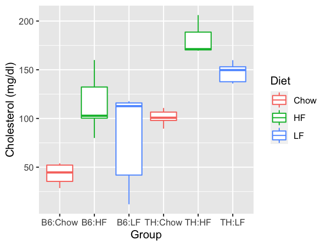
As we've seen previously, the cholesterol level in TH mice is generally higher than in B6 mice. The cholesterol level in mice fed the HF diet is generally higher than in mice fed the Chow diet. (The cholesterol level in mice fed the LF diet appears to be between the two, but there is quite a lot of variation.)

We can analyze the effect of both strain and diet on cholesterol by running a two-way ANOVA. We specify Cholesterol as a function of both Strain and Diet:


chol.strain.diet <- aov(Cholesterol ~ Strain + Diet, data=met)

This tests two hypotheses separately, but accounting for each one. Specifically, the first null hypothesis is:

The strain has no effect on the cholesterol level, if diet is held constant

and the second null hypothesis is

The diet has no effect on the cholesterol level, if strain is held constant

If we examine the summary of the two-way ANOVA:


summary(chol.strain.diet)

we see that the p-values for both strain and diet are small, indicating that we can reject both null hypotheses. I.e. both strain and diet have an effect on the cholesterol level.

We can go further than this, and examine how much effect each variable has on cholesterol:


chol.strain.diet$coefficients

To interpret the output of this:


(Intercept)    StrainTH      DietHF      DietLF 
   39.82201    63.49498    76.66237    42.82300

we need to remember how the data were set up. Both Strain and Diet are set up as factors, and the reference levels (the first levels) are B6 and Chow, respectively. (Remember, by default the levels are in alphabetical order.)

The estimate for (Intercept) represents the estimate for the cholesterol level in the reference group; i.e. in the B6 Chow group. So this ANOVA estimates the cholesterol level of a B6 mouse fed the Chow diet to be 39.82 mg.dl.

The estimate for StrainTH is the estimate for the additional level of cholesterol associated with being a TH mouse instead of a B6 mouse. So, this two-way ANOVA would estimate the cholesterol level of a TH mouse fed the Chow diet as 39.82201 + 63.49498 = 103.32 mg/dl.

The estimate for DietHF is the estimate for the additional level of cholesterol associated with a mouse being fed the HF diet (compared to the reference diet, Chow). So, this ANOVA would estimate the cholesterol level of a B6 mouse fed the HF diet as 39.82201 + 76.66237 = 116.48 mg/dl.

Similarly, the estimate for a B6 mouse fed the LF diet would be 39.82201 + 42.82300 = 82.65 mg.dl.

What about the other two groups? A TH mouse fed the HF diet would be estimated to have increases in cholesterol level over the reference group both due to being a TH mouse, and due to being fed the HF diet. Thus the estimate for cholesterol level for a TH mouse fed the HF diet from this ANOVA would be 39.82201 + 63.49498 + 76.66237 = 179.98 mg/dl.

What does this ANOVA estimate the cholesterol level of a TH mouse fed the LF diet would be (to two decimal places)?
1. 106.32 mg/dl
2. 179.98 mg/dl
3. 146.14 mg/dl
4. 159.31 mg/dl
Incorrect

The estimate for a TH mouse fed the LF diet will be the estimate for the reference group, plus the estimated effect for being a TH mouse, plus the estimated effect for being fed the LF diet.

Correct!

The estimate for a TH mouse fed the LF diet will be the estimate for the reference group, plus the estimated effect for being a TH mouse, plus the estimated effect for being fed the LF diet.

This gives 39.82201 + 63.49498 + 42.82300 = 146.14 mg/dl

We can tabulate the mean value for each group, which is fairly easy to do using tidyverse functions:


met %>% 
  group_by(Strain, Diet) %>%
  summarize(Mean_Cholesterol = mean(Cholesterol))

For comparison, the following table contains the predicted values using the estimates from the ANOVA:

Strain	Diet	Mean Cholesterol level	ANOVA estimate
B6	Chow	42.9	39.8
B6	HF	115.0	116.5
B6	LF	81.7	82.7
TH	Chow	101.0	103.3
TH	HF	182.0	180.0
TH	LF	147.0	146.14

The estimated values are close to the means for each group. The estimates minimize the total squared distance between each value in our data set, under the assumptions of the ANOVA. Note that it would be impossible to get exactly the means for each group, as there are six groups, but only four parameters in the model (Intercept, TH effect, HF effect, and LF effect).

What are these assumptions? All ANOVAs assume that the data are sampled from normally-distributed data, and that the variance in each group is equal. This two-way ANOVA, however, has an additional assumption: we assume that the effects of the two variables are independent; i.e. we are assuming that there is no interaction between these two variables. Thus, for example, to estimate the cholesterol level of a TH mouse fed the HF diet, we can consider the effects of being a TH mouse and being fed the HF diet, and just add the two effects together.

Since the estimates are close to the mean values, it seems reasonable to conclude that this model is good, i.e. that Strain and Diet are acting independently on the Cholesterol level and there is no interaction between the two variables. This is also evident in the pattern seen in the graph above: the effect of diet appears similar in the two strains (for each strain, a HF diet increases the cholesterol level, and a LF diet increases the cholesterol level over Chow, but not as much as the HF diet does).

The two-way ANOVA estimates the magnitude of these effects, and confirms what we described from graphing the data: there is an increase in cholesterol level for TH mice over B6 mice; there is an increase in cholesterol level from either HF or LF diet over the Chow diet, with the effect of the HF diet being larger than the effect of the LF diet.

We can also get confidence intervals for the magnitude of these effects:


confint(chol.strain.diet)

which gives the 95% confidence intervals for each effect:

Effect	95% confidence interval
Intercept	[17.61949, 62.02453]
StrainTH	[41.93230, 85.05767]
DietHF	[49.16562, 104.15912]
DietLF	[17.69572, 67.95028]

As in a one-way ANOVA, we are 95% confident that all these confidence intervals contains the true value of the corresponding effect.

In the next section, we'll see how to test the assumption that the variables have no interaction, and what the data and analysis look like when they do.

BMR 617: Statistical Techniques for the Biomedical Sciences

Two-Way ANOVA